
[The Monthly Mean] July/August 2011 -- What's the difference between ANOVA and ANCOVA?
The Monthly Mean is a newsletter with articles about Statistics with occasional forays into research ethics and evidence based medicine. I try to keep the articles non-technical, as far as that is possible in Statistics. The newsletter also includes links to interesting articles and websites. There is a very bad joke in every newsletter as well as a bit of personal news about me and my family.
Welcome to the Monthly Mean newsletter for July/August 2011. If you are having trouble reading this newsletter in your email system, please go to www.pmean.com/news/201107.html. If you are not yet subscribed to this newsletter, you can sign on at www.pmean.com/news. If you no longer wish to receive this newsletter, there is a link to unsubscribe at the bottom of this email. Here's a list of topics.
--> What's the difference between ANOVA and ANCOVA?
--> The dark side of search engine optimization
--> Salvaging a negative confidence interval
--> Monthly Mean Article (peer reviewed): Questions asked and answered in pilot and feasibility randomized controlled trials
--> Monthly Mean Article (popular press): How a New Hope in Cancer Fell Apart
--> Monthly Mean Book: The Statistical Evaluation of Medical Tests for Classification and Prediction
--> Monthly Mean Definition: Regression to the mean
--> Monthly Mean Quote: We must learn to count...
--> Monthly Mean Video: Career Day
--> Monthly Mean Website: Open Epi
--> Nick News: Nick ends the summer with a bang
--> Very bad joke: Actuaries are people who...
--> Tell me what you think.
--> Join me on Facebook, LinkedIn and Twitter
--> What's the difference between ANOVA and ANCOVA? ANOVA is short for ANalysis Of VAriance, and ANCOVA is short for ANalysis of COVAriance. Sometimes (rarely) you will see ANOCOVA or ANACOVA instead of ANCOVA.
Some people would argue that ANOVA and ANCOVA are trivial distinctions and that both represent specific examples of a linear regression model. The differences are that ANOVA has only categorical independent variables and ANCOVA has both categorical and continuous independent variables.
Let me try to elaborate a bit. A simple ANOVA (sometimes called one factor ANOVA) has a continuous outcome variable and a single categorical predictor variable. Depending on who you talk to, the categorical predictor variable has to have at least two or at least three different levels. I don't want to fuss too much about this, but if the categorical variable has exactly two levels, then you can use a two-sample t-test in place of an ANOVA.
The hypothesis tested by a simple ANOVA model is that the average outcome measure is the same for all levels of the categorical variable. Here's an example:
Felipe Donatto, Jonato Prestes, Anelena Frollini, Adrianne Palanch, Rozangela Verlengia, Claudia Cavaglieri. Effect of oat bran on time to exhaustion, glycogen content and serum cytokine profile following exhaustive exercise. Journal of the International Society of Sports Nutrition. 2010;7(1):32. Abstract: "The aim of this study was to evaluate the effect of oat bran supplementation on time to exhaustion, glycogen stores and cytokines in rats submitted to training. The animals were divided into 3 groups: sedentary control group (C), an exercise group that received a control chow (EX) and an exercise group that received a chow supplemented with oat bran (EX-O). Exercised groups were submitted to an eight weeks swimming training protocol. In the last training session, the animals performed exercise to exhaustion, (e.g. incapable to continue the exercise). After the euthanasia of the animals, blood, muscle and hepatic tissue were collected. Plasma cytokines and corticosterone were evaluated. Glycogen concentrations was measured in the soleus and gastrocnemius muscles, and liver. Glycogen synthetase-alpha gene expression was evaluated in the soleus muscle. Statistical analysis was performed using a factorial ANOVA. Time to exhaustion of the EX-O group was 20% higher (515 +/- 3 minutes) when compared with EX group (425 +/- 3 minutes) (p = 0.034). For hepatic glycogen, the EX-O group had a 67% higher concentrations when compared with EX (p = 0.022). In the soleus muscle, EX-O group presented a 59.4% higher glycogen concentrations when compared with EX group (p = 0.021). TNF-alpha was decreased, IL-6, IL-10 and corticosterone increased after exercise, and EX-O presented lower levels of IL-6, IL-10 and corticosterone levels in comparison with EX group. It was concluded that the chow rich in oat bran increase muscle and hepatic glycogen concentrations. The higher glycogen storage may improve endurance performance during training and competitions, and a lower post-exercise inflammatory response can accelerate recovery."[Accessed on July 18, 2011]. http://www.jissn.com/content/7/1/32
The outcome variable is time to exhaustion and the categorical predictor variable is treatment group (C, EX, or EX-O). There were differences in the means, particularly in the important comparison of the EX and EX-O groups.
A simple ANCOVA also has a continuous outcome variable, but it has two predictor variables: one categorical and one continuous. The continuous predictor variable is referred to as the covariate. There is often an unstated assumption in ANCOVA that the covariate is not of direct research interest, but rather a variable that needs to be adjusted for.
The hypothesis tested by a simple ANCOVA model is that the average outcome variable, holding the covariate constant, is the same across all levels of the categorical variable. Here's an example.
Pia Sorensen, Tom Bendix, Claus Manniche, Lars Korsholm, Dorte Lemvigh, Aage Indahl. An educational approach based on a non-injury model compared with individual symptom-based physical training in chronic LBP. A pragmatic, randomised trial with a one-year follow-up. BMC Musculoskeletal Disorders. 2010;11(1):212. Abstract: "BACKGROUND: In the treatment of chronic back pain, cognitive methods are attracting increased attention due to evidence of effectiveness similar to that of traditional therapies. The purpose of this study was to compare the effectiveness of performing a cognitive intervention based on a non-injury model with that of a symptom-based physical training method on the outcomes of low back pain (LBP), activity limitation, LBP attitudes (fear-avoidance beliefs and back beliefs), physical activity levels, sick leave, and quality of life, in chronic LBP patients. METHODS: The study was a pragmatic, single-blind, randomised, parallel-group trial. Patients with chronic/recurrent LBP were randomised to one of the following treatments: 1. Educational programme : the emphasis was on creating confidence that the back is strong, that loads normally do not cause any damage despite occasional temporary pain, that reducing the focus on the pain might facilitate more natural and less painful movements, and that it is beneficial to stay physically active. 2. Individual symptom-based physical training programme : directional-preference exercises for those centralising their pain with repetitive movements; 'stabilising exercises' for those deemed 'unstable' based on specific tests; or intensive dynamic exercises for the remaining patients. Follow-up questionnaires (examiner-blinded) were completed at 2, 6 and 12 months. The main statistical test was an ANCOVA adjusted for baseline values. RESULTS: A total of 207 patients participated with the median age of 39 years (IQR 33-47); 52% were female, 105 were randomised to the educational programme and 102 to the physical training programme. The two groups were comparable at baseline. For the primary outcome measures, there was a non-significant trend towards activity limitation being reduced mostly in the educational programme group, although of doubtful clinical relevance. Regarding secondary outcomes, improvement in fear-avoidance beliefs was also better in the educational programme group. All other variables were about equally influenced by the two treatments. The median number of treatment sessions was 3 for the educational programme group and 6 for the physical training programme group. CONCLUSIONS: An educational approach to treatment for chronic LBP resulted in at least as good outcomes as a symptom-based physical training method, despite fewer treatment sessions.TRIAL REGISTRATION: Clinicaltrials.gov: # NCT00410319" [Accessed on July 18, 2011]. http://www.biomedcentral.com/1471-2474/11/212
The outcome variable is activity limitation, the categorical predictor is treatment group, and the covariate is baseline levels of activity limitation. After adjusting for baseline differences, there was slightly less activity limitation in one of the treatment groups, although this did not achieve statistical significance.
Suppose that our covariate was categorical and not continuous. This is an ambiguous setting. Some people would still call this ANCOVA but others would call it an ANOVA with two factors. Flip a coin to decide what term you want to use here.
Did you like this article? Visit www.pmean.com/category/LinearRegression.html or www.pmean.com/category/AnalysisOfVariance.html for related links and pages.
--> The dark side of search engine optimization. Search Engine Optimization (often abbreviated SEO) is a series of methods to revise your webpages so that when someone does an Internet search for a particular topic, your page ends up at the top of the list. It's a bit of a dark art. Google and other search engines don't reveal all the details of how they rank pages based on search criteria because they don't want websites to game the system.
I get a lot of traffic on my website through Google, but I don't worry much about optimizing my site to get near the top of the Google list. When I get a high page rank for certain search terms, I'm usually pleasantly surprised. One time, though, I found out that I was near the top of list for a Google search and I was not at all happy about it.
When I was at Children's Mercy Hospital, I participated in a working group on Evidence-Based Medicine. This was an interesting and fun experience, and I got a chance to practice some skills that I was not all that good at, especially searching for the relevant evidence.
One of the exercises in this group, inspired by a true concern raised at the hospital, was about possible adverse effects of the milk with molasses enema. There were two possibilities raised. First, the explosive nature of this treatment might lead to tears or ruptures in the intestinal wall. Second, this treatment might create a serious electrolyte imbalance. One group worried a lot about these possibilities, but a competing group thought that they were just a bunch of Nervous Nellies.
I'm not a doctor, but I figured that I could do a PubMed search about as well as the others in this working group, so I did. I summarized my search strategies and my results on my website, as is my custom for anything interesting that I do. You can read this summary at
--> http://www.childrensmercy.org/stats/weblog2005/MolassesMilk.asp.
A few days later, I decided to do another search, not of the peer-reviewed literature, but of the Internet itself. You need to be very careful, of course, about Internet sources that have not been peer-reviewed, but I thought I might stumble upon something interesting or helpful.
So I ran a Google search on the three words: milk, molasses, enema. I was horrified when I found out that my own web page turned up as #3 on the Google list. I'm not a doctor, so I don't want people to think that I am an expert on medical problems. But I especially don't want to be thought of as an expert on enemas. Gack! It's worse than that because many of the sites recommended by Google were these woo-woo alternative medical sites, and there were a few pornographic stories thrown in as well.
There was something about the recency of my webpage that put me up high on the list, because as I rechecked in later weeks, my article sank down to a lower page rank. When I was no longer on the first page of Google searches, I heaved a sigh of relief.
I just checked today (July 9, 2011) and my article was back up to #4. And talking about it in this newsletter might push it even higher. Links to your webpage from authoritative outside sources often appear to help your page rank. I'm not sure if Google considers The Monthly Mean as an authoritative source though. I'm not so worried anymore. If anyone tries to contact me via Children's Mercy, they will probably end up getting to my former boss, a Clinical Pharmacologist. Let him worry about being perceived as an expert on enemas.
Did you like this article? Visit http://www.pmean.com/category/InformationSearching.html for related links and pages.
--> Salvaging a negative confidence interval. Dear Professor Mean, I was involved in a small case-control project that was intended to explore some genotypes as predictors of disease progression. We had between 50 and 60 cases and controls (each). One particular predictor had a OR of 0.5 with 95% confidence limits of 0.2 and 1.2. We reported the negative results, but a a long time a go, I did read some papers showing some different interpretations of confidence intervals. If I remember right, there was some statements like: it is less likely that a point estimate such as 0.5[0.2-1.2] be 1 then one as 0.8[0.5-1.2], considering the proportion of the CI that is distant from 1. Even now, it sounds weird to me. Can I say something about this in my paper?
I've often said that once scientists get a p-value less than 0.05 or a confidence interval that implies statistical significance, they turn their brains off. You've got a confidence interval that implies lack of statistical significance and a p-value larger than 0.05 so your brain is still churning away. That's good, but all the thinking you are doing now to "salvage" a negative study should be applied equally to trying to place appropriate limitations on a positive study.
I might be a bit simplistic, but rather than the hypothetical intervals you propose, let me propose something a bit more extreme. A confidence interval that goes from 0.7 to 1.2 is pretty definitive example of a negative finding, because this interval excludes any clinically interesting odds ratios. The confidence interval that goes from 0.2 to 1.2, though does have the "advantage" of being ambiguous because it allows you to claim that something interesting might still be going on. Here I'm deliberately making the mistake that only positive findings are interesting.
Now I should state that sometimes an odds ratio of 0.8 is clinically relevant, but let's assume that only more extreme odds ratios such as 0.67 and 1.5 are clinically important for this particular problem.
The problem, of course, is that an odds ratio confidence interval of 0.2 to 0.8 has all the problems of the interval 0.2 to 1.2. Both intervals contain both clinically important and clinically trivial values but people never treat the former interval as being ambiguous. So what if an odds ratio of 0.75 implies that the new treatment cannot be justified based on the extra costs and side effects that come with the new treatment? I've got a statistically significant finding, so I don't need to be pestered with any bad thoughts.
The only time people wrestle with borderline findings is when they are on the "wrong" side of the border. P-values of 0.048 and 0.052 are probably saying pretty much the same thing, but only the latter gets any serious discussion. If you run around jumping and hollering enough, maybe you can jostle that 0.052 enough that it jumps to the other side. That 0.048 though is delicate and perilously close to falling off the cliff into the sea of statistical non-significance. So we'll be very quiet and tiptoe cautiously around that p-value lest we ruin our happy mood at obtaining a positive study.
Don't let me stop you from talking about your non-significant finding though. Too many people treat a p-value larger than 0.05 as a gag rule and limit their discussion only to those tests and confidence intervals yielding statistically significant results. That's a far worse sin than trying to salvage a negative confidence interval.
Did you like this article? Visit www.pmean.com/category/ConfidenceIntervals.html for related links and pages.
--> Monthly Mean Article (peer reviewed): Milensu Shanyinde, Ruth Pickering, Mark Weatherall. Questions asked and answered in pilot and feasibility randomized controlled trials. BMC Medical Research Methodology. 2011;11(1):117. Abstract: "BACKGROUND: In the last decade several authors have reviewed the features of pilot and feasibility studies and advised on the issues that should be addressed within them. We extend this literature by examining published pilot/feasibility trials that incorporate random allocation, examining their stated objectives, results presented and conclusions drawn, and comparing drug and non-drug trials. METHODS: A search of EMBASE and MEDLINE databases for 2000 to 2009 revealed 3652 papers that met our search criteria. A random sample of 50 was selected for detailed review. RESULTS: Most of the papers focused on efficacy: those reporting drug trials additionally addressed safety/toxicity; while those reporting non-drug trials additionally addressed methodological issues. In only 56% (95% confidence intervals 41% to 70%) were methodological issues discussed in substantial depth, 18% (95% confidence interval 9% to 30%) discussed future trials and only 12% (95% confidence interval 5% to 24%) of authors were actually conducting one. CONCLUSIONS: Despite recent advice on topics that can appropriately be described as pilot or feasibility studies the large majority of recently published papers where authors have described their trial as a pilot or addressing feasibility do not primarily address methodological issues preparatory to planning a subsequent study, and this is particularly so for papers reporting drug trials. Many journals remain willing to accept the pilot/feasibility designation for a trial, possibly as an indication of inconclusive results or lack of adequate sample size." [Accessed on September 3, 2011]. http://www.biomedcentral.com/1471-2288/11/117.
Did you like this article? Visit www.pmean.com/category/PilotStudies.html for related links and pages.
--> Monthly Mean Article (popular press): Gina Kolata. How a New Hope in Cancer Fell Apart. The New York Times. July 7, 2011. Excerpt: "The episode is a stark illustration of serious problems in a field in which the medical community has placed great hope: using patterns from large groups of genes or other molecules to improve the detection and treatment of cancer. Companies have been formed and products have been introduced that claim to use genetics in this way, but assertions have turned out to be unfounded. While researchers agree there is great promise in this science, it has yet to yield many reliable methods for diagnosing cancer or identifying the best treatment." [Accessed on July 9, 2011]. http://www.nytimes.com/2011/07/08/health/research/08genes.html.
Did you like this article? Visit www.pmean.com/category/DiagnosticTesting.html for related links and pages.
--> Monthly Mean Book: Margaret Sullivan Pepe. The Statistical Evaluation of Medical Tests for Classification and Prediction (Oxford Statistical Science Series). Excerpt from the back cover: "The use of clinical and laboratory information to detect conditions and predict patient outcomes is a mainstay of medical practice. This book describes the statistical concepts and techniques for evaluating the accuracy of medical tests. Main topics include: estimation and comparison of measures of accuracy, including receiver operating characteristic curves; regression frameworks for assessing factors that influence test accuracy and for comparing tests while adjusting for such factors; and sample size calculations and other issues pertinent to study design. Problems relating to missing and imperfect reference data are discussed in detail. Additional topics include: meta-analysis for summarizing the results of multiple studies of a test; the evaluation of markers for predicting event time data; and procedures for combining the results of multiple tests to improve classification. A variety of worked examples are provided. [This book] will be of interest to quantitative researchers and to practicing statisticians. The book also covers the theoretical foundations for statistical inference and will be of interest to academic statisticians."
Did you like this book? Visit www.pmean.com/category/DiagnosticTesting.html for related links and pages.
--> Monthly Mean Definition: What is regression to the mean? Dear Professor Mean, In a stat course I was introduced to the term "regression to the mean". Today we administered a pretest to 4th graders. In Feb we will again test, with the same exam, to see "how much they've learned". I explained to the principal that, of course they would do better, no matter how well they were taught, that this was a classic case of regression to the mean. Am I correct, close, or way off on this?
You're half right, but Professor Mean doesn't give partial credit.
Regression to the mean can explain how individuals behave, but it does not usually characterize how groups of individuals behave. The one exception is when the group is selected on the basis of one of the variables.
It might help to remember the application where the concept of regression to the mean was first discovered. Sir Francis Galton was interested in the relationship between a child's height (when the child reaches adulthood) and the height of the parents. There are several ways to look at the data: the height of the father versus the height of the child, the height of the mother versus the height of the child, or the average height of both parents versus the height of the child.
One example, described on page 169 of Friedman, Pisani and Purves (1998), examines the relationship between the height of the father and the height of a male child. For this data, the correlation was 0.5. When you look at the prediction equation, though, the results at first seem a bit counterintuitive. Without knowing anything else, you might expect that the best prediction for a male child's height would be the father's height. In other words, if the father is 74 inches, your best prediction of the male child's height would also be 74 inches.
It doesn't quite work out that way, partly because the average child's height (69 inches) was one inch greater than the average father's height (68 inches). That may be due to better nutrition or some other environmental factor. Both groups did have the same standard deviation, though (2.7).
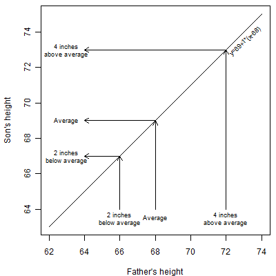
The graph shown above shows what you might think would happen. An average father (68 inches) is expected to have an average son (69 inches). This is not a fixed height. Some of the sons are going to be 70 or 72 inches and some are going to be 66 or 68 inches. But these will balance out in the long run to an average of 69 inches. You'd also expect an above average dad to have above average sons. You'd expect a dad that is 72 inches (four inches above dad average of 68 inches) for example to have a son that is around 73 inches (four inches above the son average of 69 inches). Again we're not expecting every son to be exactly 73 inches. This is just an average tendency. Likewise a dad that is 66 inches (two inches below the dad average of 68 inches) would be expected to have a 67 inch son (two inches below the son average of 67 inches).
The linear equation for these ideal predictions would be y = 69 + 1 * (x - 68)
In actuality, the equation for predicting son's expected height from the dad's height is y = 69 + 0.5 * (x - 68). That equation is illustrated below.
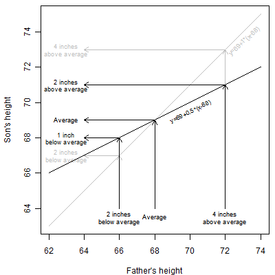
In this equation, an average dad (68 inches) will be still expected to have an average son (69 inches). But a dad that is 72 inches (four inches above the dad average) will be expected to have a 71 inch son. That is still above the son average of 69 but it is only two inches above average, half of the dad's four inch excess. So above average dads will tend to produce above average sons, but the height excess is attenuated. The effect in below average dads is also interesting. A dad that is 66 inches (two inches below the dad average) will be expected to have a 68 inch son. That's still below average, but the one inch deficit in height in the son is half the size of the two inch deficit in the dad.
This seems counterintuitive. If each son is moving towards the mean, wouldn't the successive generations converge to a single height? The trick is that there are random deviations from the expected heights. These random deviations spread out the actual heights of the sons to compensate for the regression to the mean. In fact, if there weren't regression to the mean, then the variation in successive generations would explode.
I should note here that it is just a coincidence that the expected surplus or deficit is cut exactly in half. The size of the regression to the mean effect depends on the correlation between the two variables being studied. Depending on the problem the regression to the mean effect could be stronger than this example or it could be weaker.
The same general tendencies hold, by the way, when you look at the mother's height, or the average of father's and mother's height. It also holds when you look at the heights of daughters.
Things get a bit messier when the outcome or dependent variable is in different units than the predictor variable. In these settings, it helps to think in terms of standardized variables.
Now what are the practical implications of regression to the mean?
In the testing example that you give, suppose the average student scores 50 at the start of classes and 70 at the end of classes. Then regression to the mean will tell you how much students deviate from the mean of 70 at the end of classes on the basis of how much they deviated from the mean of 50 at the beginning of classes.
A student who is one standard deviation above the average score of 50 at the start of classes is probably going to be a bit less than a full standard deviation above average score of 70 at the end of classes. So you might be a bit disappointed with "smart" students.
A student who is one standard deviation below the average score of 50 at the start of classes is probably going to be a bit less than one standard deviation below the average score of 70 at the end of classes. You might get encouraged by "dumb" students.
Where regression to the mean tends to cause unexpected results is when you select students on the basis of their pre-test values. For example, a naive researcher might split a sample of students into a "smart" class and a "dumb" class on the basis of a preliminary test. There might be, say a 10 point gap between the two groups based on the preliminary test. But all other things being equal, you should expect the gap between the "smart" and the "dumb" class to be narrower by the end of the year.
Of course, you don't use terms like "smart" and "dumb" for your students. The point here is that if you segregate students on the basis of their performance at the start of the class, the amount the two groups appear to learn at the end of classes will vary even if nothing else differs between the two groups.
Regression to the mean also can appear in medical settings. Quite often we will segregate patients into "sick" and "healthy" categories on the basis of some medical test. If we re-tested these groups at a later date, we would probably see that the "sick" category probably isn't quite as sick as we thought they were and the "healthy" category probably isn't as healthy as we thought they were.
Suppose we measure cholesterol levels in 100 patients and select the 50 patients with above average cholesterol levels for a special diet and exercise program. Even if that program were entirely ineffective, you would probably see some level of cholesterol reduction. The change would have been balanced out by the 50 patients in the below average group who would probably show an increase on average if we had taken the time and trouble to follow them as well.
Sometimes patients will self-select themselves for a new treatment. Some illnesses are cyclical, with random peaks and troughs in how the patient feels. Patients are most likely to adopt a new approach (change doctors, discontinue medication, etc.) when they are in a trough. When the inevitable rebound occurs, the patient might falsely attribute the rebound to the change in treatment. This is especially true when the patient focuses on a small time scale. In fact, regression to the mean is one of the many causes of the placebo effect in medicine.
Some processes show a natural progression in the averages, and we would expect a roughly similar progression in individual values. For example, almost all children grow--short children grow and tall children grow too. So, for example, a three year old child with a height above the average of all three year olds will, after a year, grow (maybe a little and maybe a lot). This pretty much guarantees that, at the age of four, this child will be even farther above the average height of all three year olds. That's not surprising and it is not a contradiction of regression to the mean. What you have to do, of course, is to look at that child's four year old height relative to all four year old children.
Also, regression to the mean for individuals on the low end will tend to balance out regression to the mean for individuals on the high end. So, if you select an average or unremarkable group of individuals, and there is no preferential selection of individuals above average and no screening or exclusion of individuals who are below average, then that group, as a whole, will not exhibit regression to the mean.
Finally, regression to the mean is a statistical tendency, so there will always be exceptions. There will be some individuals who are above average at baseline and even more above average at the end of the study. It's also possible, once in a while for an entire group to move in a direction opposite of what regression to the mean would tell you. After all, any time you have randomness, unpredictable things can happen.
This article is an update of something I wrote for my old website:
-->
http://www.childrensmercy.org/stats/ask/regression.asp
Did you like this article? Visit http://www.pmean.com/category/StatisticalTheory.html for related links and pages.
--> Monthly Mean Quote: We must learn to count the living with that same particular attention with which we number the dead. Audre Lorde, as quoted in The Emperor of All Maladies: A Biography of Cancer, Siddhartha Mukherjee.
--> Monthly Mean Video: Career Day. A three minute clip from That 70's Show where Kelso's dad, a statistician, tries to explain what he does. http://www.youtube.com/watch?v=KjkGizs84rE
--> Monthly Mean Website: AG Dean, KM Sullivan, MM Soe. OpenEpi: Open Source Epidemiologic Statistics for Public Health, Version 2.3.1. Excerpt: "OpenEpi provides statistics for counts and measurements in descriptive and analytic studies, stratified analysis with exact confidence limits, matched pair and person-time analysis, sample size and power calculations, random numbers, sensitivity, specificity and other evaluation statistics, R x C tables, chi-square for dose-response, and links to other useful sites." [Accessed on June 28, 2011]. http://www.openepi.com/OE2.3/Menu/OpenEpiMenu.htm.
Did you like this website? Visit http://www.pmean.com/category/StatisticalComputing.html for related links and pages.
--> Nick News: Nick ends the summer with a bang. Nicholas is back in school, but the 30 days before school started were quite eventful. Here's an update of everything that happened with a few pictures.
As mentioned earlier, we got a dog, Cinnamon. Cinnamon loves to chew on things, and it is a constant struggle to keep our house and belongings intact. Nick just loves Cinnamon and plays with her constantly.

Nick had his ninth birthday. He invited some friends over for a swim party and a sleepover. Half of them had already arrived and Nick was showing them his scooter. He hit a bump and landed face first into the concrete. Cathy took Nick to the Urgent Care Center at Children's Mercy South and Steve had to keep the kids who were there entertained at the pool. Nick came back with six stitches under his chin, but he was still able to eat cake and host the sleepover.

Two days after Nick's birthday, Steve had to leave for a business trip to Miami Beach. The air conditioning was acting a bit goofy before he left, but it quit completely once he was gone. Cathy had to cope with no air conditioning when the temperatures were all in the danger level. The worst day had a temperature of 106.
Also while Steve was gone, Nick had his stitches removed (also at Children's Mercy South), but the wound site didn't heal up as quickly as we would have hoped. When Nick bumped his chin on the bannister, the wound re-opened and he had to visit Children's Mercy South for the third time in one week. Steve arrived home as this was happening and met Nick and Cathy at the Urgent Care room. Nick was quite good, possibly because it was late and he was tired. He fell asleep while they were working on a more comprehensive set of stitches.
A couple of days after Steve returned, we all took a trip to Colorado. We rented a condo in Avon, which is up in the mountains near Vail and Beaver Creek.

The three of us rode down from Vail Pass on bikes. See more pictures of the Colorado trip at
--> http://www.pmean.com/personal/summer.html
--> Very bad joke: Actuaries are people who decided to liven up the rather boring subject of Statistics by combining it with Insurance. This is an original joke of mine. When I was in high school and all through my undergraduate time at the University of Iowa, I knew that I wanted to be an actuary. It took one course in my first semester of graduate school to convince me that Actuarial Science was not the career for me.
--> Tell me what you think. How did you like this newsletter? Give me some feedback by responding to this email. Unlike most newsletters where your reply goes to the bottomless bit bucket, a reply to this newsletter goes back to my main email account. Comment on anything you like but I am especially interested in answers to the following three
questions.
--> What was the most important thing that you learned in this newsletter?
--> What was the one thing that you found confusing or difficult to follow?
--> What other topics would you like to see covered in a future newsletter?
I received feedback from four people. One liked the article on McNemar's test, though the topic was a bit difficult to follow. I also got positive feedback on Ten Commandments for Fellows, secondary outcome measures, and rates versus proportions. Oh, I also got two positive comments on the picture of my son and his new dog. They make a very cute pair, don't they?
There was one suggestion about the admonition of using change scores in a parallel groups pre-test/post-test design. This is a very tricky area, and I don't agree with the consensus opinion. It might be hard for me to write such an article, but I'll try.
--> Join me on Facebook, LinkedIn, and Twitter. I'm just getting started with social media. My Facebook page is www.facebook.com/pmean, my page on LinkedIn is www.linkedin.com/in/pmean, and my Twitter feed name is @profmean. If you'd like to be a Facebook friend, LinkedIn connection, or tweet follower, I'd love to add you. If you have suggestions on how I could use these social media better, please let me know.
What now?
Sign up for the Monthly Mean newsletter
Review the archive of Monthly Mean newsletters
![]() This work is licensed under a
Creative
Commons Attribution 3.0 United States License. This page was written by
Steve Simon and was last modified on
2017-06-15. Need more
information? I have a page with general help
resources. You can also browse for pages similar to this one at
Category: Website details.
This work is licensed under a
Creative
Commons Attribution 3.0 United States License. This page was written by
Steve Simon and was last modified on
2017-06-15. Need more
information? I have a page with general help
resources. You can also browse for pages similar to this one at
Category: Website details.