[Previous issue] [Next issue]
Monthly Mean newsletter, March/April 2009
The monthly mean for March/April is 15.25. It's been a busy couple of months so I might have to change this to the Bimonthly Mean. Actually, I'm hoping to return to a
monthly schedule for May.
Welcome to the Monthly Mean newsletter for March/April 2009. If you are having
trouble reading this newsletter in your email system, please go to www.pmean.com/news/2009-03.html. If you are not yet subscribed to this
newsletter, you can sign on at www.pmean.com/news. If you no longer wish to receive this newsletter, there is a link to unsubscribe at the bottom
of this email. Here's a list of topics.
- Lead article: Help! My sample size is too small!
- Research scientists are truly are special people
- Help! My research study is behind schedule!
- Monthly Mean Article: Relation of study quality, concordance, take home
message, funding, and impact in studies of influenza vaccines: systematic
review
- Monthly Mean Blog: Radford Neal's blog
- Monthly Mean Book: Missing Data: A Gentle Introduction
- Monthly Mean Definition: Generalized Estimating Equations
- Monthly Mean Quote: The best thing about being a statistician...
- Monthly Mean Website: Negative Consequences of Dichotomizing Continuous
Predictor Variables
- Nick News: Nicholas the scientist
- Very bad joke: How many research subjects does it take to screw in a
lightbulb?
- Tell me what you think.
1. Lead article: Help! My sample size is too small!
I get a lot of inquiries, directly and indirectly, from people who want to
start a research project, but they know that their sample size is too small. A
common question is along the lines of what test can I use for a sample size of
5 that will guarantee statistical significance. I tell them that they need to use the "blood from a turnip" test.
Actually, you can't guarantee statistical significance, even with a sample
size of 5,000. What a larger sample size provides is greater credibility both in
a qualitative sense and a quantitative sense.
Many of the people who review the results of your data analysis will not
trust the results if they come from a small sample size. It's hard to say how
small is too small to lose credibility, because it varies from area to area and
from person to person. But I've seen a healthy suspicions of small sample sizes
from most of the researchers that I have worked with. Perhaps this suspicion is
overly healthy; I've seen people express reservations about sample sizes that
were actually quite adequate.
A larger sample size also provides greater credibility in a quantitative
sense. The confidence intervals produced by larger sample sizes are much more
precise than those produced by small samples (all other things being equal, of
course). A story I tell people about why you should worry about sample size involves a
research who gets a 6 year, 10 million dollar grant. At the end of the 6 years,
he writes a report that reads "This is a new and innovative surgical procedure,
and we are 95% confident that the cure rate is somewhere between 3% and 98%."
So what factors go into getting an adequate sample size? The first is
typically a power calculation. In some situations, an alternative way to
determine sample size is by specifying the desired width of the confidence
intervals produced by the research. An inadequate sample size produces too
little power or too imprecise confidence intervals.
Ensuring adequate power or adequate precision
is only part of the battle. In a randomized experiment with heterogenous
subjects, some chance imbalances can still occur. For the same reason that ten
flips of a coin is not a guarantee that you will get exactly five heads and five
tails, a randomization of 10 subjects is no guarantee that both the good and poor
prognosis patients will be evenly divided between the treatment group and
the control group. Randomization relies on the law of large numbers and it takes
a fairly large sample size to insure that you get a good balance
among a group of heterogenous subjects. With a single important covariate, a
total sample size of 20 works well, but if you have two or three important
covariates, 80 may be required. This is less of a concern in animal experiments and laboratory experiments
where great efforts are taken to insure consistency from one sampling unit to
another.
Finally, the complexity of the statistical model will often require a sample
size larger than your budget might allow. There's an informal rule that you need
at least 10 observations per independent variable in any regression model.
Sometimes you will see the rule being cited as 15 observations per independent
variable, and other sources have even suggested 20 observation per independent
variable. This widely cited rule has been applied to
linear regression, logistic regression, and other types of
regression models. If you try to search for the original justification for this
rule, you will find that it is based on a logistic regression model. Although
there is no reason to believe that the rule would not apply equally well to a
linear regression model or a Cox regression model, I am unaware of any formal study of this rule in
these
regression models.
In a logistic regression model, it is actually a bit more strict. You need 10
to 15 events (not observations) per independent variable. So if you collect 1,000 observations, but
only observe 60 events, then you should only consider a model with 4 to 6
independent variables.
One quick caveat. If you have 5 potential confounders and 3 of
them turn out to be non-significant, you have not improved your events per
variable ratio. The
very process of screening or evaluating a covariate causes the problem,
whether or not it survives the final cut using stepwise approaches or anything
similar. If you look at a variable at any time during the data analysis phase
(excluding trivial descriptive statistics), then it counts towards your events
per variable
ratio. The only ways to improve this ratio is to
- increase your sample size and thus your number of events, or
- eliminate some confounders during the planning phase (before any data is
collected).
During the planning phase of some studies, you might be able to change the
population being studied in order to increase the number of events. If your
event is something bad like relapse or rehospitalization, then collecting data
from a more seriously ill population would increase the proportion of events in
your sample, leading to greater power and precision for a given sample size. It
may seem callous, but statisticians need to have a lot of bad things happen in
order to have something worth studying. If you collect data on 20,000 patients,
and there are four deaths in the control group and two deaths in the treatment
group, you have cut the risk of mortality in half, but there is no way that you
can make statistical sense of this limited amount of information.
In a highly heterogenous situation or a situation with several important
covariates (essentially the same thing), you should consider matching or
stratification in the design stage, if it's not too late. There are also some
new statistical methods that work well with screening a large number of
potential covariates. I will try to summarize some of these methods in future
newsletters.
In summary, there are three different rules that can help determine if your
sample size is adequate: a power or precision calculation, a minimum of 80
subjects to ensure proper randomization in a highly heterogenous population, and
a minimum of 10 to 15 observations/events per independent variable. If you have
a problem with one of these criteria, it doesn't matter if the other two
criteria are satisfied or not.
If you've already collected a data set with an inadequate sample size, it was
either out blissful ignorance or a willful disregard. I'm not sure which one is
worse, but I hope you're hanging your head in shame right now.
In either case, you should
still try to publish your data. Don't compound the sin of collecting an
inadequate sample with another sin of contributing to publication bias. Just be honest in your
methods section by saying that no power calculation was conducted prior to data
collection. Some people have argued that you should conduct a power calculation
after the data is already collected. This type of power calculation, called a
post hoc power calculation, is actually a very bad idea. Instead, be sure to
include confidence limits for all of your key estimates. The embarrassingly wide
intervals will provide a much better clue to your readers about the impact of
your inadequate sample size.
If you are in the planning stages and you recognize that your sample size
is too small, ask yourself whether collecting this data, with all its
limitations, is worth the trouble. You don't want to spend 10 million dollars
of someone else's money and then only give them a confidence interval of 3% to
98% in return.
2. Research scientists are truly special people
The Kansas City Star (our local newspaper) had an article about how the
recent financial stimulus package passed by the U.S. Congress has a lot of money
to expand research, and gave some examples of research efforts in the local area
would benefit from this work. I decided to submit an article for the editorial
page elaborating on my experiences working with researchers. They are almost
uniformly great people to work with.
The Star decided not to publish my article, so here it is for your benefit.
If you are a research scientist, pat yourself on the back after reading this.
You deserve it
Your article "Science Finds an Ally in Obama" (page B1, Monday, March 2)
extols the virtues of research, but does not go nearly far enough. As a
professional statistician, I have had the pleasure of working with research
scientists in many different disciplines, and these people are truly wonderful
to work with.
Researchers are extremely industrious, working far harder than I ever could.
There are no "banker's hours" in the scientific community. I've tagged along as
a scientist made a special evening trip to the lab just to make an extra
infusion in their cell line. I've gotten emails well beyond midnight from
scientists needing feedback from a just finished a research proposal (I never
admit that I am playing FreeCell when I get these messages). I've had to
schedule some of my meetings as early as 7am to accommodate medical
professionals who see a full slate of patients during normal clinic hours. I did
draw the line at a researcher who suggested a Saturday morning meeting. No one
is taking my Saturday morning cartoons away from me.
Researchers are highly altruistic. They see problems and want to fix them. I
have countless examples of this, but one is particularly memorable because I am
so squeamish. I was working with a doctor investigating the use of ultrasound
during kidney biopsies to make them safer and less painful. One of the biggest
benefits that he was able to demonstrate was the reduction in the number of
biopsies that had to be redone. I cringe at the thought of a needle going into
my kidney. I can't imagine getting it done and then having the doctor say,
whoops, we didn't get enough tissue, do you mind if we do it again?
Researchers also have a refreshing sense of humility. A true scientist knows
that ideas aren't valid just because they were thought up by someone who gets
paid to do a lot of thinking. To be worth anything, research hypotheses have to
be proven with cold hard data. When the data points in a different direction,
researchers swallow their pride and abandon their cherished hypotheses. I've
seen this happen many times and it is not pleasant. It's worse than simply
admitting a mistake because it does not happen in private. Scientific progress
requires that negative findings be publicized to prevent others from going down
the same blind alley. It takes a truly humble person to admit in a research
publication that they had a great idea, but when it was carefully tested it
proved to be totally wrong.
We need more research. I do have a conflict of interest here--more research
means more people seeking my services for data analysis. But any objective
analysis of research funding should recognize its benefits. Research projects
require lots of labor and the jobs produced are high quality jobs. But more than
this, research leads to saved lives and better quality of life. Research
scientists are truly the unsung heroes of our country.
3. Help! My research study is behind schedule!
Research always seems to take longer than you expect. You hope to get
enough patients in a year's time, but after two years, you aren't even halfway
to your target sample size. There has been a lot written about determining an
appropriate sample size, but relatively little about the accrual rate, the
speed at which you are able to obtain this sample size.
I have been working with Byron Gajewski to develop a model to
plan an appropriate accrual rate for an upcoming clinical trial and to monitor
that rate as patients join the study to see if your study is still on a good
time line. If patients are joining your trial too slowly, this model will
provide a revised estimate of when you will be able to finish recruiting the
desired number of subjects.
I won't show the mathematical details here, but the accrual model relies on an exponential
waiting time between successive patients. You can find all the formulas at
- Gajewski BJ, Simon SD, Carlson S. "Predicting accrual in clinical trials
with Bayesian posterior predictive distributions" Statistics in Medicine
(2008): 27(13); 2328-2340. DOI: 10.1002/sim.3128 [Medline] [Abstract].
A similar accrual model based on the Poisson distribution was developed
independently and published a few months earlier in the same journal
- Anisimov VV, Fedorov VV. "Modelling, prediction and adaptive adjustment
of recruitment in multicentre trials" Statistics in Medicine (2007); 26:
4958-4975. DOI: 10.1002/sim.2956 [Medline] [Abstract].
We've adopted a Bayesian approach for this model, which means that you must
specify a prior distribution on the mean waiting time. There is a belief among some critics of Bayesian Statistics that the prior
distribution allows subjective beliefs to be incorporated into an otherwise
objective analysis. A true scientist should be disinterested in the results of
the research so as to maintain the credibility of the research findings. There
are several counterarguments to this criticism, of course, and others can make
these counter-arguments better than I can.
From the perspective of accrual, however, there should be no debate. A
researcher would never undertake a clinical trial unless he/she had a least an
inkling of how quickly patients would volunteer for the trial. Soliciting such
beliefs does no harm to the supposed objectivity of the final data analysis.
In fact, you can use a Bayesian model for accrual for a clinical trial where
all of the proposed data summaries are classical non-Bayesian.
The big advantage to specifying a prior distribution is that when a
researcher has extensive experience in given research arena and provides
appropriately precise prior distributions, that will prevent the researcher
from overreacting to a bit of early bad news about accrual. In contrast when a
researcher provides only a vague prior distribution about accrual patterns,
early evidence of problems is given greater weight, allowing for rapid
interventions to correct the slow accrual.
Eliciting a prior distribution is a difficult task. We start our elicitation
by asking two simple questions
- How long will it take to accrue n subjects?
- On a scale of 1-10, how confident are you in your answer to 1?
There are several methods to examine the reasonableness of the prior
distribution and to possibly refine it which we discuss briefly in the article.
Eliciting a good prior distribution is an art.
To illustrate the proposed method, consider an unnamed current phase III
clinical trial (randomized, double-blind, and placebo-controlled) used to
examine the efficacy and safety of a dietary supplement. This study was planned
and accrual started prior to our development of these methods, but still serves
to illustrate how this approach would work. The current protocol requires n=350
subjects, with balanced randomization to either treatment or placebo control. In
the previous study, investigators were able to recruit, from a similar
population, 350 subjects across 3 years. The average waiting time was set at 3.1
days (3*365/350). The previous experience with a similar set of patients
suggests a reasonably strong prior distribution (5 on a scale of 1 to 10).
With this prior distribution, the researcher can predict the trial duration
and account for uncertainty in the accrual rate and
uncertainty due to the random nature of the exponential accrual model.

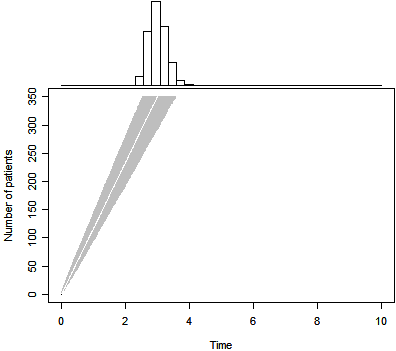
The graph above shows the predicted trial duration based solely on the prior
distribution. The gray region represents the range between the 2.5 and 97.5
percentiles. The white line in the middle of this region represents the 50th
percentile.
For this particular prior distribution, the 50th percentile for trial
duration is 3.0 years. There is a 0.025 probability that the trial could finish
in 2.5 years or less and a 0.025 probability that it could last 3.6 years or
longer.
After the study was funded and the protocol approved, the investigative team
began recruiting subjects. After 239 days the project director compiled a report
that displays enrolled dates of 41 subjects. This represents an average waiting
time of 5.8 days, much longer than prior expectation (3.1 days).

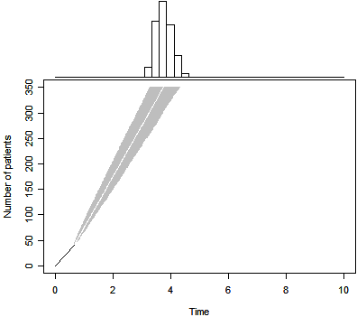
The Bayesian prediction appears above. Notice that the estimated
completion time is not a simple linear projection of the data, as the prior
distribution still exerts enough influence to bend the projection back slightly.
The 50th percentile for trial duration is 3.7 years, a substantial increase over
the original belief that the trial would last about 3 years. The 2.5 and 97.5
percentiles for the Bayesian predictive distribution are 3.3 and 4.3. so even
allowing for the uncertainties in the accrual pattern, there is a very high
probability that this trial will finish later than planned.

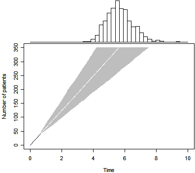
We can produce a Bayesian predictive distribution for a non-informative prior
as well. The results are shown above. Note that the median trial duration (5.6
years) is now a simple linear projection of the accrual trend through the first
41 subjects. This approach, however, properly accounts for the uncertainty
associated with this trend. The 2.5 and 97.5 percentiles are 4.2 and 7.5
years respectively.
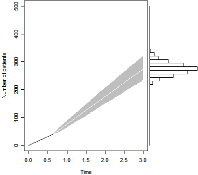
Let's use the same prior distribution, but produce a
simulation that estimates the final sample size under the assumption that the
trial must end at exactly 3 years.

The figure above shows the projected sample size after 239 days
and 41 patients. The median is 274, and the 2.5 and 97.5
percentiles (233 and 321 respectively) are both well below the original
expectation of recruiting 350 patients.
The R code for producing these graphs is available at my old website.
It is fairly easy for you to examine more complex accrual
patterns, such an accrual goal of recruiting until 50 patients have volunteered,
or until 6 months have elapsed, whichever comes first.
The model we propose is easily extended in a variety of
ways:
- Use of alternatives to the exponential distribution for modeling waiting
times.
- Examination of alternative prior distributions.
- Use hierarchical models to predict accrual across multiple centers in a
multi-center trial.
This Bayesian model looks very promising and if anyone reading this
newsletter wants to try it on their own research, please contact me for help.
4. Monthly Mean Article: Relation of study quality, concordance, take home
message, funding, and impact in studies of influenza vaccines: systematic review
Jefferson T, Di Pietrantonj C, Debalini MG, Rivetti A, Demicheli V.
Relation of study quality, concordance, take home message, funding, and impact
in studies of influenza vaccines: systematic review. BMJ.
2009;338(feb12_2):b354. Available at:
www.bmj.com/cgi/content/abstract/338/feb12_2/b354 [Accessed March 31,
2009].
These authors identified 259 published studies of influenza vaccines and
rated these studies according to their funding source and the take-home message.
Additional information was collected to assess the quality of the research. The
authors also examined whether the take home message was actually consistent with
the data presented.
This latter point is important but underappreciated. Many times researchers
will state conclusions that are not supported by the data and sometimes they
will state conclusions that are flat out contradicted by the data. You would
think that the peer-review process would prevent this from happening, but sad to
say, there is still a lot of this going on. It might be self-delusion of the
researchers or it might be a conscious effort to "spin" the data a certain way.
In any case, it is a warning that you should read more than just the discussion
and conclusion of a paper.
To help understand this better, the authors present three papers where there
is inconsistency between the data presented and the conclusions drawn.
Comment: though authors state that effectiveness is shown for influenza
related ARI only, and not influenza, they recommend vaccination for patients
with COPD. This means recommending vaccine though it is not effective against
influenza and acute exacerbations. In addition, lack of comment on community
viral circulation and vaccine content and matching make verification of
effectiveness against ARI impossible.
Comment: influenza vaccination is recommended though outcomes are
exclusively serological (surrogates) calculated in aggregate over three years
(180 in intervention arms and 179 in three different control arms). Clinical
outcomes are not significantly affected by vaccination.
Comment: implausible conclusion with use of all cause mortality an outcome
lacking specificity. Long list of confounders: biased reporting of autopsy
sampling, trenchant conclusion despite apparent lack of effect on viral
circulation, brief description of vaccine content or matching (in discussion),
attrition in serology follow-up, possible selection bias of healthcare workers
and patients, higher Barthel score in vaccinated arm.Once data were adjusted for
Barthel score, age, and sex no effect was observed.
The researchers showed that higher quality studies were much less likely to
present unsupported results. This could mean that researchers who were careful
enough to use a good research design were also careful enough to portray their
data accurately. Or it might mean that the less rigorous research designs are
also more complex and difficult to understand, leading to a greater degree of
unsupported conclusions.
Industry funded studies were no better methodologically than other studies
(government funded or funding source unknown), but they were far more likely to
be published in high impact journals. Industry funded studies appear to be more
likely to have a supportive take home message, but the wording of the article is
a bit confusing on this point.
This study is important because it shows not only the tendency for industry
support to "buy" favorable conclusions, but also the ability to publish those
favorable conclusions in more prominent journals. The authors only touch on this
lightly, but industry sponsored research often leads to the same industry
purchasing and redistributing massive numbers of reprints. Since purchase of
reprints is a major source of income for many journals, there is the potential
for journals to preferentially publish industry sponsored studies to improve
their bottom line. Such a potential conflict of interest would not exist for an
open source publication.
5. Monthly Mean Blog: Radford Neal's blog
Neal R. Radford Neal's blog. Available at:
radfordneal.wordpress.com/ [Accessed March 13, 2009]. Radford
Neal is one of the superstars of the statistics world, and his blog is just
getting started. It covers some high powered stuff, so this is not for the
dabbler in statistics. He talks about the design flaws in R (#1,
#2, and
#3),
a decision theory approach to fetal testing for Down's syndrome, and
coverage issues for frequentist confidence intervals.
6. Monthly Mean Book: Missing Data: A Gentle Introduction
McKnight PE, McKnight KM, Sidani S, Figueredo AJ. (2007) Missing Data: A
Gentle Introduction. New York, NY: The Guilford Press. I just bought this book
recently. It is one of the rare statistics books available on my Amazon Kindle.
So far, it is an excellent read. These four authors are social scientists who
were confused by the existing literature on missing values, so they did what any
smart person would do. They organized a series of talks about missing data at
the American Evaluation Association conference of 1994. This is my general
approach, as well. If you find something difficult, try to teach it to an
audience who knows as little about it as you do. Your efforts to make the issue
understandable to them will make it understandable to yourself at a level that
can't be rivaled by other approaches.
The book has a mellow pace to it that is
illustrated by a comment in the preface "At the heart of it all, we embrace a
philosophy where researchers calmly approach missing data as an interesting
question rather than as a catastrophe".
The authors have an admirable chapter on preventing missing data, a pragmatic
topic that is ignored by many textbooks. They cover both simple methods, such as
complete case analysis, and complex methods, such as multiple imputation.
Although their goal to produce a book without a lot of mathematics prevents the
reader from getting the complete details of how to implement the more complex
procedures, these details are readily available elsewhere. You will instead
learn when and why you would want to use the more complex procedures, a far more
important lesson.
7. Monthly Mean Definition: Generalized Estimating Equations
Generalized Estimating Equations (GEE) are a statistical model that is an
extension of the Generalized Linear Model (GLM). They could have called it the
Generalized Generalized Linear Model (GGLM), but that would be confusing. Like
GLM, GEE can analyze data from a normal model (linear regression), a binomial
model (logistic regression), a Poisson model (Poisson regression), and other
models as well. GEE has additional capability beyond GLM because it can
analyze data from a longitudinal design, a cluster randomized design, or other
designs where correlations among some of the observations are allowed. GEE
is able to handle unbalanced data, such as longitudinal designs with different
number of time points for different subjects, or different cluster sizes. If you
use a GEE model, you need to specify a pattern for the correlations across time
or within a cluster. It is important from an efficiency perspective to try to
specify the correlation pattern correctly, but the GEE
model uses an approach that is valid even if the pattern you select for the
correlations is incorrect. There is an alternative approach for longitudinal
designs and cluster randomized trials, going by several different names, the
hierarchical linear model, mixed linear regression models, and random
coefficient models.
8. Monthly Mean Quote: The best thing about being a statistician...
"The best thing about being a statistician is that you get to play in
everyone's backyard." -- John W Tukey, as quoted at
www.geocities.com/damaratung/.
9. Monthly Mean Website: Negative Consequences of Dichotomizing Continuous
Predictor Variables.
McClelland, Gary. Negative Consequences of Dichotomizing Continuous Predictor
Variables. Available at:
psych.colorado.edu/~mcclella/MedianSplit/ [Accessed January 8, 2009].
It's popular in some research areas to take a continuous predictor variable
and turn it into a binary predictor variable. Often the research will define the
binary variable as 1 if the continuous variable is above the median and 0 if it
is below the median. This forces the binary variable to have equal numbers in
the two categories (unless you live in Lake Wobegon, where all the children are
above average).
A median split sometimes simplifies the interpretation of the research results,
but there is a price to be paid. A binary variable does not have any "shades of
gray" because any values just below the median are treated the same as values
far below the median. Values just above the median are treated the same as vales
well above the median. The median split leads to a loss of information and
results in a less efficient statistical model. Gary McClelland has a nice Java
applet that visually shows the loss of information. Take the slider bar at the
bottom of the graph and move it from a truly continuous variable all the way to
the other side where it is replaced by a median split. The regression line
flattens out, the p-value increases, and for this particular example, you lose
statistical significance. This applet is a fun way to illustrate an important
point.
10. Nick News: Nicholas the scientist
At Nicholas's school, there is an afterschool program called "Science Stars."
We weren't sure if Nicholas would like this, but we signed him up. It has been
very successful in at least one aspect, he now says it's his favorite part of
school. Until recently, his favorite parts of school were either gym or recess.

Here, Nicholas is holding "flubber"
or what I used to know as "silly
putty." It's supposed to show something about polymers, but I think
most kids like it because you can squish it and bounce it. Go to
to see more pictures of Nicholas's scientific explorations.
11. Very bad joke: How many research subjects does it take to screw in a lightbulb?
This is an original joke by me. It was published at my old website:
www.childrensmercy.org/stats/size/power.asp
How many research subjects does it take to screw in a lightbulb? At least
300 if you want the bulb to have adequate power.
12. Tell me what you think.
How did you like this newsletter? I have three short open ended questions
that I'd like to ask. It's totally optional on your part. Your responses will
be kept anonymous, and will only be used to help improve future versions of
this newsletter.
I got only one response to my feedback webpage. The respondent was relieved
by my comments about small sample sizes, a reaction I had not expected.
"The small samples problem isn't a big as i thought it was -- I worry
about paediatric trials with 20-30 patients, but shouldn't so much."
The entry was "Is there a sample size too small to allow efficient
randomization?" and it is only one of several considerations. I elaborate on this in more detail in this month's newsletter. Still, if
you're able to conduct a research study with 20-30 patients and get good
precision on your confidence intervals, don't let anyone convince you that
your sample size is too small.
That person also asked for more material on generalized estimating
equations (GEE), and other closely related topics. I've added a definition of
GEE in this newsletter and hope to show some examples of various models in
this area in future newsletters.
I did get some nice compliments by email. Thanks! I'd brag about all the nice things you've said, but my email folders are in limbo thanks to a malfunctioning laptop.
What now?
Sign up for the Monthly Mean newsletter
Review the archive of Monthly Mean newsletters
Take a peek at an early draft of the next
newsletter
Go to the main page of the P.Mean website
Get help
 This work is licensed under a
Creative
Commons Attribution 3.0 United States License. This page was written by
Steve Simon and was last modified on
2017-06-15.
