Illustrating splines using the Worcester Heart Attack Study

*Blog post
2024
Incomplete pages
Survival analysis
R programming
Uses R code
Author

Steve Simon

Published

May 7, 2024

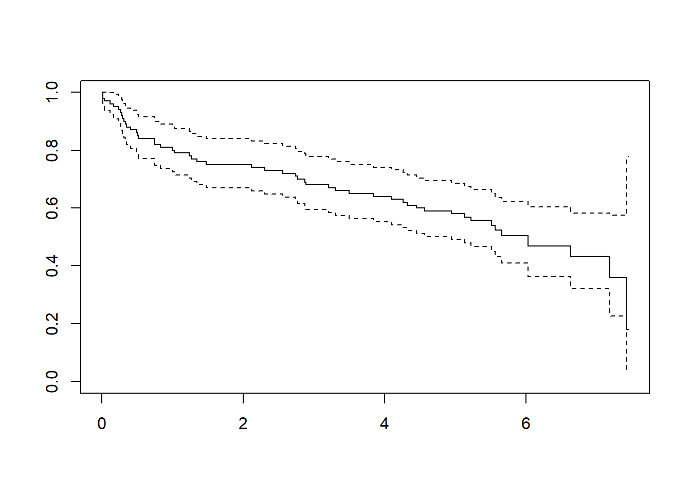
Splines provide a useful way to model relationships that are more complex than a simple linear relationship. They work in a variety of regression models. Here is an illustration of how to use a spline in a Cox regression model with data from the Worcester Heart Attack Study.

Here is a brief description of the whas100 dataset, taken from the data dictionary on my github site.

The data represents survival times for a 100 patient subset of data from the Worcester Heart Attack Study. You can find more information about this data set in Chapter 1 of Hosmer, Lemeshow, and May.

Here are the first few rows of data and the last few rows of data. Row 101 needs to be removed.

  id    admitdate      foldate los lenfol fstat age gender    bmi
1  1 03/13/1995   03/19/1995     4      6     1  65      0 31.381
2  2 01/14/1995   01/23/1996     5    374     1  88      1 22.650
3  3 02/17/1995   10/04/2001     5   2421     1  77      0 27.878
4  4 04/07/1995   07/14/1995     9     98     1  81      1 21.478
5  5 02/09/1995   05/29/1998     4   1205     1  78      0 30.706
6  6 01/16/1995   09/11/2000     7   2065     1  82      1 26.452
     id    admitdate      foldate los lenfol fstat age gender    bmi
96   96 11/04/1997   12/31/2002     4   1883     0  48      1 32.117
97   97 12/24/1997   04/19/2002     3   1577     1  32      1 39.938
98   98 11/26/1997   01/27/1998     8     62     1  86      1 14.918
99   99 08/10/1997   12/31/2002    16   1969     0  56      0 29.052
100 100 03/26/1997   02/13/2000     7   1054     1  74      0 32.890
101  NA         <NA>         <NA>  NA     NA    NA  NA     NA     NA

Here are a few descriptive statistics

   Min. 1st Qu.  Median    Mean 3rd Qu.    Max. 
   1.00   25.75   50.50   50.50   75.25  100.00 
   Min. 1st Qu.  Median    Mean 3rd Qu.    Max. 
   1.00    4.00    5.00    6.84    7.00   56.00 
   Min. 1st Qu.  Median    Mean 3rd Qu.    Max. 
0.01643 1.95756 5.14031 4.12156 5.68515 7.44422 
  fstat  n
1     0 49
2     1 51
   Min. 1st Qu.  Median    Mean 3rd Qu.    Max. 
  32.00   59.75   71.00   68.25   80.25   92.00 
  gender  n
1      0 65
2      1 35
   Min. 1st Qu.  Median    Mean 3rd Qu.    Max. 
  14.92   23.54   27.19   27.04   30.35   39.94 

Here is an overall survival curve.

plot(Surv(wa$lenfol, wa$fstat))

The linear fit shows a hazard ratio larger than 1. The risk of death increases with age.

linear_fit <- coxph(
  Surv(wa$lenfol, wa$fstat)~age,
  data=wa)
linear_fit
Call:
coxph(formula = Surv(wa$lenfol, wa$fstat) ~ age, data = wa)

       coef exp(coef) se(coef)     z        p
age 0.04567   1.04673  0.01195 3.822 0.000132

Likelihood ratio test=17.36  on 1 df, p=3.09e-05
n= 100, number of events= 51 

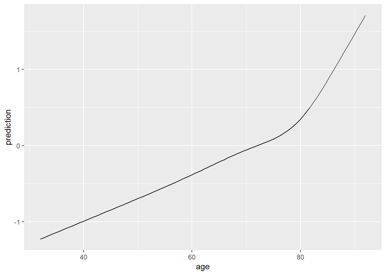
The coefficients of the spline fit are impossible to interpret. It is better to view the spline fit graphically.

spline_fit <- coxph(
  Surv(wa$lenfol, wa$fstat)~rcs(age),
  data=wa)
number of knots in rcs defaulting to 5
spline_fit
Call:
coxph(formula = Surv(wa$lenfol, wa$fstat) ~ rcs(age), data = wa)

                    coef exp(coef)  se(coef)      z     p
rcs(age)age     0.029460  1.029898  0.057288  0.514 0.607
rcs(age)age'    0.007734  1.007764  0.178424  0.043 0.965
rcs(age)age''  -0.073750  0.928903  1.077082 -0.068 0.945
rcs(age)age'''  0.582372  1.790279  2.134665  0.273 0.785

Likelihood ratio test=19.77  on 4 df, p=0.0005539
n= 100, number of events= 51 

The risk of death increases linearly with age up to about 80 years and then take a sharp curve upward. This shows that each additional year of age beyond 80 has a large impact on survival, much larger than additional years of age earlier in life.

age_sequence <- data.frame(
  age = seq(min(wa$age), max(wa$age), length=100))
age_sequence$prediction <- 
  predict(spline_fit, newdata=age_sequence, type="lp")
ggplot(data=age_sequence, aes(age, prediction)) +
  geom_line()