  id age gender hr sysbp diasbp      bmi cvd afb sho chf av3 miord mitype year
1  1  83      0 89   152     78 25.54051   1   1   0   0   0     1      0    1
2  2  49      0 84   120     60 24.02398   1   0   0   0   0     0      1    1
3  3  70      1 83   147     88 22.14290   0   0   0   0   0     0      1    1
4  4  70      0 65   123     76 26.63187   1   0   0   1   0     0      1    1
5  5  70      0 63   135     85 24.41255   1   0   0   0   0     0      1    1
6  6  70      0 76    83     54 23.24236   1   0   0   0   1     0      0    1
   admitdate    disdate      fdate los dstat lenfol fstat
1 01/13/1997 01/18/1997 12/31/2002   5     0   2178     0
2 01/19/1997 01/24/1997 12/31/2002   5     0   2172     0
3 01/01/1997 01/06/1997 12/31/2002   5     0   2190     0
4 02/17/1997 02/27/1997 12/11/1997  10     0    297     1
5 03/01/1997 03/07/1997 12/31/2002   6     0   2131     0
6 03/11/1997 03/12/1997 03/12/1997 1 1 1 1The lasso model allows you to effectively identify important features in a large regression model. Here is an illustration of how to use a the lasso model with survival data from the Worcester Heart Attack Study.
I’ve followed the glmnet vignette for Cox regression closely. You might find that explanation to be clearer than what I present below.
Description of the whas500 dataset
Here is a brief description of the whas500 dataset, taken from the data dictionary on my github site.
The data represents survival times for a 500 patient subset of data from the Worcester Heart Attack Study. You can find more information about this data set in Chapter 1 of Hosmer, Lemeshow, and May.
Here are the first few rows of data and the last few rows of data. Row 101 needs to be removed.
Here are a few descriptive statistics
gender: gender
  gender   n
1      0 300
2      1 200

cvd: History of Cardiovascular Disease
  cvd   n
1   0 125
2   1 375

afb: Atrial Fibrillation
  afb   n
1   0 422
2   1  78

sho: Cardiogenic Shock
  sho   n
1   0 478
2   1  22

chf: Congestive Heart Complications
  chf   n
1   0 345
2   1 155

av3: Complete Heart Block
  av3   n
1   0 489
2   1  11

miord: MI Order
  miord   n
1     0 329
2     1 171

mitype: MI Type
  mitype   n
1      0 347
2      1 153

year: Cohort Year
  year   n
1    1 160
2    2 188
3    3 152

dstat: Discharge Status from Hospital
  dstat   n
1     0 461
2     1  39

fstat: Vital Satus
  fstat   n
1     0 285
2     1 215
age: Age at Admission
age
Min. : 30.00
1st Qu.: 59.00
Median : 72.00
Mean : 69.85
3rd Qu.: 82.00
Max. :104.00
hr: Initial Heart Rate
hr
Min. : 35.00
1st Qu.: 69.00
Median : 85.00
Mean : 87.02
3rd Qu.:100.25
Max. :186.00
sysbp: Initial Systolic Blood Pressure
sysbp
Min. : 57.0
1st Qu.:123.0
Median :141.5
Mean :144.7
3rd Qu.:164.0
Max. :244.0
diasbp: Initial Diastolic Blood Pressure
diasbp
Min. : 6.00
1st Qu.: 63.00
Median : 79.00
Mean : 78.27
3rd Qu.: 91.25
Max. :198.00
bmi: Body Mass Index
bmi
Min. :13.05
1st Qu.:23.22
Median :25.95
Mean :26.61
3rd Qu.:29.39
Max. :44.84
los: Length of Hospital Stay
los
Min. : 0.000
1st Qu.: 3.000
Median : 5.000
Mean : 6.116
3rd Qu.: 7.000
Max. :47.000
lenfol: Follow Up Time
lenfol
Min. : 1.0
1st Qu.: 296.5
Median : 631.5
Mean : 882.4
3rd Qu.:1363.5
Max. :2358.0 Simple analysis
I am going to show the R code from this point onward so you can see the actual programming required to fit a lasso model.
Here is an overall survival curve.
plot(Surv(w1$lenfol, w1$fstat))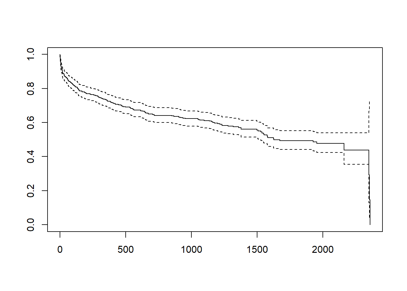
Here is the traditional Cox model
simple_fit <- coxph(
  Surv(w1$lenfol, w1$fstat) ~
      cvd +
      afb +
      sho +
      chf +
      av3 +
      miord +
      mitype,
    data=w1)
coef(simple_fit)
cvd afb sho chf av3 miord
-0.13512116 0.12295437 1.17397718 1.13970970 0.03502956 0.25505995
mitype
-0.75381851 The lasso model
You can find the lasso regression model in the glmnet package. One important difference with glmnet is that it does not use a formula to define your model. Instead you provide matrices for your dependent variable and your independent variables. In a Cox regression model, the dependent matrix has a column for time and a second column with an indicator variable (1 means the event occurred and 0 means censoring).
ymat <- cbind(w1$lenfol, w1$fstat)
dimnames(ymat)[2] <- list(c("time", "status"))
xmat <- as.matrix(w1[ , 8:14])
dimnames(xmat)[2] <- list(vnames[8:14])
lasso_fit <- glmnet(xmat, ymat, family="cox", standardize=FALSE)
plot(lasso_fit, xvar="lambda", label=TRUE)
Let’s spend a bit of time looking at this graph. The left hand side of the graph represents a very small penalty.
fit_left <- as.matrix(coef(lasso_fit, min(lasso_fit$lambda)))
fit_left
1
cvd -0.1045003
afb 0.1151425
sho 1.1199680
chf 1.1288924
av3 0.0000000
miord 0.2387614
mitype -0.7244685plot(lasso_fit, xvar="lambda", label=TRUE)
text(
log(min(lasso_fit$lambda)),
fit_left,
unlist(dimnames(fit_left)[1]))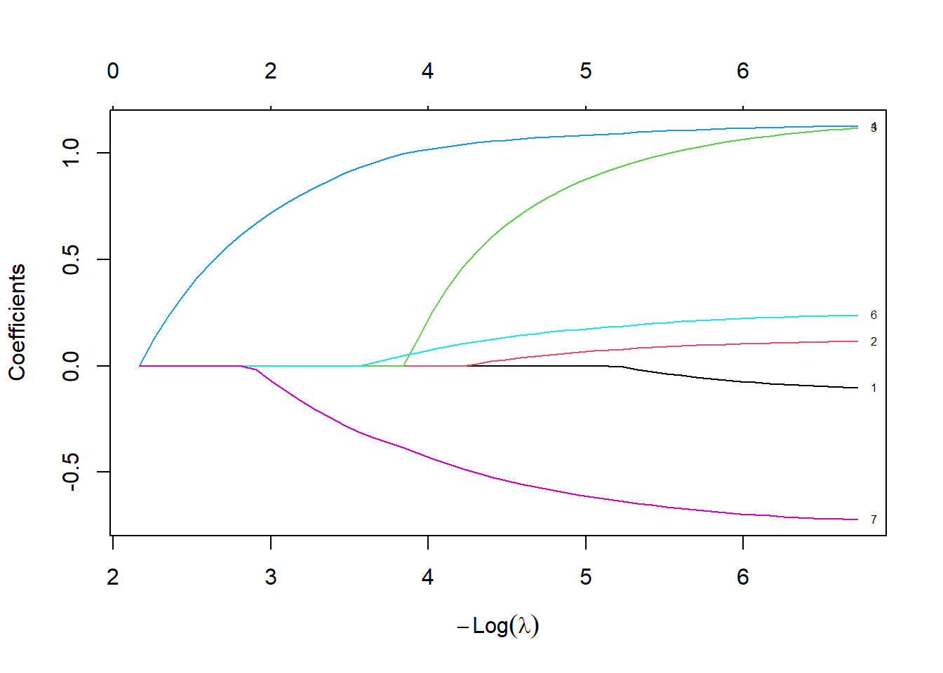
Notice how the coefficients are very close to the Cox regression model. There is very little shrinkage and only one variable, av3, are zeroed out, meaning that it is totally removed from the model.
fit_median <- as.matrix(coef(lasso_fit, median(lasso_fit$lambda)))
fit_median
1
cvd 0.00000000
afb 0.02505858
sho 0.63270940
chf 1.05928764
av3 0.00000000
miord 0.12988143
mitype -0.53060276plot(lasso_fit, xvar="lambda", label=TRUE)
text(
log(median(lasso_fit$lambda)),
fit_median,
unlist(dimnames(fit_median)[1]))
At the middle (median) value of lambda, several of the variables are zeroed out. Most other variables are shrunk towards zero, relative to the fit with the smallest value of lambda.
What happens at the largest value of lambda?
fit_right <- as.matrix(coef(lasso_fit, max(lasso_fit$lambda)))
fit_right
1
cvd 0
afb 0
sho 0
chf 0
av3 0
miord 0
mitype 0plot(lasso_fit, xvar="lambda", label=TRUE)
text(
log(max(lasso_fit$lambda)),
fit_right,
unlist(dimnames(fit_right)[1]))
Once lambda gets large enough, the penalty is so great that the algorithm zeroes out every single variable.
Cross-validation to select the optimal value of lambda
Now you need to decide what lambda works best. You can do this through cross-validation.
cv_fit <- cv.glmnet(xmat, ymat, family = "cox", standardize=FALSE)
plot(cv_fit)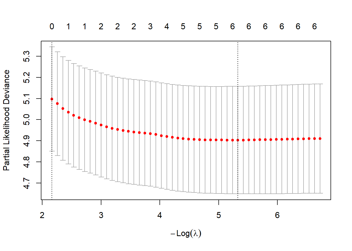
There are two choices that are commonly selected.
You could set the value of lambda to the value that minimizes the criteria. The default criteria is the partial likelihood deviance, but you can use other criteria to pick out the “best” value of lambda.
cv_fit$lambda.min[1] 0.004855224plot(lasso_fit, xvar="lambda")
abline(v=log(cv_fit$lambda.min))
fit_min <- as.matrix(coef(lasso_fit, cv_fit$lambda.min))
fit_min 1
cvd -0.01737968
afb 0.08333976
sho 0.96283217
chf 1.09896576
av3 0.00000000
miord 0.19388646
mitype -0.64692124text(log(cv_fit$lambda.min), fit_min, unlist(dimnames(fit_min)[1]))
The developers of glmnet felt that the value of lambda that minimized a fit criteria was not aggressive enough in zeroing out and shrinking coefficients. They suggested that instead of choosing the “best” value of lambda, choose the largest value of lambda that is still within one standard error of the criteria produced by the “best” lambda.
plot(lasso_fit, xvar="lambda", label=TRUE)
abline(v=log(cv_fit$lambda.1se))
cv_fit$lambda.1se
[1] 0.1148013fit_1se <- as.matrix(coef(lasso_fit, cv_fit$lambda.1se))
fit_1se 1
cvd 0
afb 0
sho 0
chf 0
av3 0
miord 0
mitype 0text(log(cv_fit$lambda.1se), fit_1se, unlist(dimnames(fit_1se)[1]))
Using this criteria, there are only two variables which help in predicting risk of death, and one of them is very weak because its coefficient is very close to zero.