This page is currently being updated from the earlier version of my website. Sorry that it is not yet fully available.
I recently heard about a contest sponsored by Revolution Analytics. Revolution Analytics is offering $20,000 in prizes to the best examples of applying R to business problems. This competition is designed to grow the collection of on-line materials describing how to use R, and to spur adoption of R and Revolution R for business applications. The contest is open to all R users worldwide. http://www.inside-r.org/howto/enter. I want to submit the R code that I developed for the accrual paper published by Byron Gajewski and me in 2008.
My submission is still an early draft, but you can look at it at –> http://www.inside-r.org/howto/predict-duration-your-clinical-trial
The R code was originally published at –>http://www.pmean.com/08/ExponentialAccrual.aspx
but I have tweaked it a bit here.
duration.plot <- function(n,T,P,m,tm,B=1000,Tmax=2*T,sample.paths=0) {
#
# n is the target sample size
# T is the target completion time
# P is the prior certainty (0 <= P <= 1)
# m is the sample observed to date
# tm is the time to date
# B is the number of simulated duration times
# Tmax is the upper limit on the time axis of the graph
#
# set P to zero for a non-informative prior
# set m and tm to zero if no data has been accumulated yet.
  k <- n*P+m
  V <- T*P+tm
#
# Draw B samples from the inverse gamma distribution
  theta <- 1/rgamma(B,shape=k,rate=V)
#
# Create and fill a matrix of simulated trial durations
  simulated.duration <- matrix(NA,nrow=n-m,ncol=B)
  for (i in 1:B) {
    wait <- rexp(n-m,1/theta[i])
    simulated.duration[,i] <- tm+cumsum(wait)
  }
#
# Each column is a separate simulated trial of waiting
# times for the remaining n-m patients. Calculate quantiles
# across the rows to get confidence limits on the waiting
# times for patients m+1, m+2, ..., n.
  lcl <- apply(simulated.duration,1,quantile,probs=0.025)
  mid <- apply(simulated.duration,1,quantile,probs=0.500)
  ucl <- apply(simulated.duration,1,quantile,probs=0.975)
#
# Graph the simulated accruals. Create a layout with two graphs
# The top graph is a histogram of the total estimated accrual for
# the full trial. The bottom graph is a display of predicted
# waiting times for patients m+1, m+2, ..., n.
  layout(matrix(c(1,2,2,2)))
#
# No margins on bottom, top, and right of histogram.
  par(mar=c(0.1,4.1,0.1,0.1))
#
# create histogram with 40 bars.
  duration.hist <- cut(simulated.duration[n-m,],
    seq(0,Tmax,length=40))
  barplot(table(duration.hist),horiz=FALSE,
    axes=FALSE,xlab=" ",ylab=" ",space=0,
    col="white",names.arg=rep(" ",39))
#
# No margins on boot, top, and right of graph of waiting
# times for patients m+1, m+2, ..., n.
  par(mar=c(4.1,4.1,0.1,0.1))
#
# Layout graph and axes, but no data yet.
  plot(c(0,Tmax),c(0,n),xlab="Time",
    ylab="Number of patients",type="n")
#
# Draw a polygon in gray ranging from lower to upper
# quantile limits.
  polygon(c(lcl,rev(ucl)),c((m+1):n,n:(m+1)),
    density=-1,col="gray",border=NA)
#
# Draw a white line at the median.
  lines(mid,(m+1):n,col="white")
#
# Draw a black line showing observed accrual through patient m.
  segments(0,0,tm,m)
#
# Draw a samll number of simulated accrual pathways
  while (sample.paths>0) {
    lines(simulated.duration[,sample.paths],(m+1):n)
    sample.paths <- sample.paths-1
  }
#
# Calculate and return percentiles to estimated total accrual time.
  pctiles <- matrix(NA,nrow=2,ncol=3)
  dimnames(pctiles) <- list(c("Waiting time","Trial duration")
    ,c("2.5%","50%","97.5%"))
  pctiles[1,] <- 1/qgamma(c(0.975,0.5,0.025),shape=k,rate=V)
  pctiles[2,1] <- lcl[n-m]
  pctiles[2,2] <- mid[n-m]
  pctiles[2,3] <- ucl[n-m]
  list(pct=pctiles,sd=simulated.duration)
}
The function calls that produced the three figures shown below are
p0 <- duration.plot(n=350,T=3,P=0.5,m= 0,tm= 0,Tmax=10)
p1 <- duration.plot(n=350,T=3,P=0.5,m=41,tm=239/365,Tmax=10)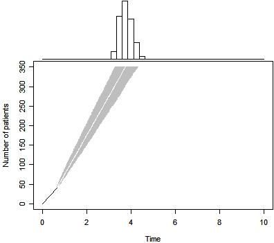
p2 <- duration.plot(n=350,T=3,P=0, m=41,tm=239/365,Tmax=10)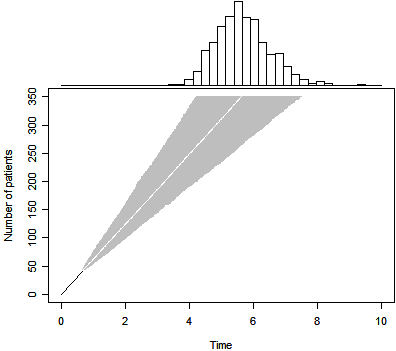
The due date for a submission is October 31.