library(lubridate)
library(mapproj)
# library(rgeos)
library(rjson)
library(rnaturalearth)
library(rnaturalearthdata)
library(rnaturalearthhires)
library(sf)
library(stringr)
library(tidyverse)I have been drawing some maps in R and was struggling to figure out how to display things with the appropriate map projections. Here is some code where I experimented with a variety of approaches.
The earth is a three dimensional object and there is no way to display it on a two dimensional computer screen without some distortion. Your goal is to minimize that distortion.
First things first. There are a variety of map options, and they have a variety of storage methods.
One of the tutorials I viewed had mentioned Natural Earth, an open source repository. You can get easy access to this information with two R packages: rnaturalearth and rnaturalearthdata.
What these give you is the ability to draw outlines of any and every country. You also get the outlines of states/provinces/districts in many countries. There’s a lot more, but I want to just show something simple now to get you started.
Note: the package, naturalearthhires is also needed for this program, but naturalearthhres is not available through CRAN. You have to use a different approach to install it.
The traditional format for storing map information is shapefiles. The shapefile format was defined the 1990s and is a rather intimidating collection of multiple files. You can find a nice summary on the Wikipedia page on shapefiles or at a Library of Congress’s page on archival formats.
A newer format, simple features, has greater flexibility and a simpler structure. It’s still not simple, and I have been able to delve into the inner workings to get important details extracted.
There is a package in R, sf, that allows you to easily manipulate geographic data stored in a simple features format. This package has a nice series of vignettes, starting here.
Please note that the rnaturalearthhires package is needed below, but it cannot be downloaded directly (at least on my system). Instead you have to type in the command
install.packages("rnaturalearthhires", repos="http://packages.ropensci.org", type="source")So to get everything to work, even for a simple example, you need a whole bunch of packages. Here are the ones I use in this example.
I’m going to read in the United States file using the ne_states function. The country=“United States of America” parameter excludes other countries that have states, provinces, or districts. I further want to remove Alaska and Hawaii from the file. So sorry to our 49th and 50th states, but the graphs are much more manageable for these examples when I focus just on the 48 states. The str function tells you a bit of information about how the data is organized within the states data frame.
ne_states(country="United States of America", returnclass = "sf") %>%
  filter(postal == "CO") -> co
str(co)
Classes 'sf' and 'data.frame': 1 obs. of 122 variables:
$ featurecla: chr "Admin-1 states provinces lakes"
$ scalerank : int 2
$ adm1_code : chr "USA-3522"
$ diss_me : int 3522
$ iso_3166_2: chr "US-CO"
$ wikipedia : chr "http://en.wikipedia.org/wiki/Colorado"
$ iso_a2 : chr "US"
$ adm0_sr : int 1
$ name : chr "Colorado"
$ name_alt : chr "CO|Colo."
$ name_local: chr NA
$ type : chr "State"
$ type_en : chr "State"
$ code_local: chr "US08"
$ code_hasc : chr "US.CO"
$ note : chr NA
$ hasc_maybe: chr NA
$ region : chr "West"
$ region_cod: chr NA
$ provnum_ne: int 0
$ gadm_level: int 1
$ check_me : int 20
$ datarank : int 1
$ abbrev : chr "Colo."
$ postal : chr "CO"
$ area_sqkm : int 0
$ sameascity: int -99
$ labelrank : int 0
$ name_len : int 8
$ mapcolor9 : int 1
$ mapcolor13: int 1
$ fips : chr "US08"
$ fips_alt : chr NA
$ woe_id : int 2347564
$ woe_label : chr "Colorado, US, United States"
$ woe_name : chr "Colorado"
$ latitude : num 39
$ longitude : num -106
$ sov_a3 : chr "US1"
$ adm0_a3 : chr "USA"
$ adm0_label: int 2
$ admin : chr "United States of America"
$ geonunit : chr "United States of America"
$ gu_a3 : chr "USA"
$ gn_id : int 5417618
$ gn_name : chr "Colorado"
$ gns_id : int -1
$ gns_name : chr NA
$ gn_level : int 1
$ gn_region : chr NA
$ gn_a1_code: chr "US.CO"
$ region_sub: chr "Mountain"
$ sub_code : chr NA
$ gns_level : int -1
$ gns_lang : chr NA
$ gns_adm1 : chr NA
$ gns_region: chr NA
$ min_label : num 3.5
$ max_label : num 7.5
$ min_zoom : num 2
$ wikidataid: chr "Q1261"
$ name_ar : chr "كولورادو"
$ name_bn : chr "কলোরাডো"
$ name_de : chr "Colorado"
$ name_en : chr "Colorado"
$ name_es : chr "Colorado"
$ name_fr : chr "Colorado"
$ name_el : chr "Κολοράντο"
$ name_hi : chr "कॉलराडो"
$ name_hu : chr "Colorado"
$ name_id : chr "Colorado"
$ name_it : chr "Colorado"
$ name_ja : chr "コロラド州"
$ name_ko : chr "콜로라도"
$ name_nl : chr "Colorado"
$ name_pl : chr "Kolorado"
$ name_pt : chr "Colorado"
$ name_ru : chr "Колорадо"
$ name_sv : chr "Colorado"
$ name_tr : chr "Colorado"
$ name_vi : chr "Colorado"
$ name_zh : chr "科罗拉多州"
$ ne_id : num 1.16e+09
$ name_he : chr "קולורדו"
$ name_uk : chr "Колорадо"
$ name_ur : chr "کولوراڈو"
$ name_fa : chr "کلرادو"
$ name_zht : chr "科羅拉多州"
$ FCLASS_ISO: chr NA
$ FCLASS_US : chr NA
$ FCLASS_FR : chr NA
$ FCLASS_RU : chr NA
$ FCLASS_ES : chr NA
$ FCLASS_CN : chr NA
$ FCLASS_TW : chr NA
$ FCLASS_IN : chr NA
$ FCLASS_NP : chr NA
$ FCLASS_PK : chr NA
$ FCLASS_DE : chr NA
[list output truncated]
- attr(*, "sf_column")= chr "geometry"
- attr(*, "agr")= Factor w/ 3 levels "constant","aggregate",..: NA NA NA NA NA NA NA NA NA NA ...
..- attr(*, "names")= chr [1:121] "featurecla" "scalerank" "adm1_code" "diss_me" ...names(co) [1] "featurecla" "scalerank" "adm1_code" "diss_me" "iso_3166_2"
[6] "wikipedia" "iso_a2" "adm0_sr" "name" "name_alt"
[11] "name_local" "type" "type_en" "code_local" "code_hasc"
[16] "note" "hasc_maybe" "region" "region_cod" "provnum_ne"
[21] "gadm_level" "check_me" "datarank" "abbrev" "postal"
[26] "area_sqkm" "sameascity" "labelrank" "name_len" "mapcolor9"
[31] "mapcolor13" "fips" "fips_alt" "woe_id" "woe_label"
[36] "woe_name" "latitude" "longitude" "sov_a3" "adm0_a3"
[41] "adm0_label" "admin" "geonunit" "gu_a3" "gn_id"
[46] "gn_name" "gns_id" "gns_name" "gn_level" "gn_region"
[51] "gn_a1_code" "region_sub" "sub_code" "gns_level" "gns_lang"
[56] "gns_adm1" "gns_region" "min_label" "max_label" "min_zoom"
[61] "wikidataid" "name_ar" "name_bn" "name_de" "name_en"
[66] "name_es" "name_fr" "name_el" "name_hi" "name_hu"
[71] "name_id" "name_it" "name_ja" "name_ko" "name_nl"
[76] "name_pl" "name_pt" "name_ru" "name_sv" "name_tr"
[81] "name_vi" "name_zh" "ne_id" "name_he" "name_uk"
[86] "name_ur" "name_fa" "name_zht" "FCLASS_ISO" "FCLASS_US"
[91] "FCLASS_FR" "FCLASS_RU" "FCLASS_ES" "FCLASS_CN" "FCLASS_TW"
[96] "FCLASS_IN" "FCLASS_NP" "FCLASS_PK" "FCLASS_DE" "FCLASS_GB"
[101] "FCLASS_BR" "FCLASS_IL" "FCLASS_PS" "FCLASS_SA" "FCLASS_EG"
[106] "FCLASS_MA" "FCLASS_PT" "FCLASS_AR" "FCLASS_JP" "FCLASS_KO"
[111] "FCLASS_VN" "FCLASS_TR" "FCLASS_ID" "FCLASS_PL" "FCLASS_GR"
[116] "FCLASS_IT" "FCLASS_NL" "FCLASS_SE" "FCLASS_BD" "FCLASS_UA"
[121] "FCLASS_TLC" "geometry" There is a lot of information in the list above and more than half of it is just giving different names to each state. The last column in this data frame is geometry and this is going to be the last column of any data stored in the simple features format. It ends up being a very long string with latitude and longitude coordinates for one or more polygons. You need multiple polygons for a disconnected state like Michigan, or a state with a lot of islands, like Florida.
Similarly, the ne_countries function gets information about the boundaries of every country in the world.
countries <- ne_countries(scale = "medium", returnclass = "sf")
str(countries)
Classes 'sf' and 'data.frame': 242 obs. of 169 variables:
$ featurecla: chr "Admin-0 country" "Admin-0 country" "Admin-0 country" "Admin-0 country" ...
$ scalerank : int 1 1 1 3 5 6 1 1 1 3 ...
$ labelrank : int 3 3 3 2 3 6 4 3 4 6 ...
$ sovereignt: chr "Zimbabwe" "Zambia" "Yemen" "Vietnam" ...
$ sov_a3 : chr "ZWE" "ZMB" "YEM" "VNM" ...
$ adm0_dif : int 0 0 0 0 0 0 0 0 0 0 ...
$ level : int 2 2 2 2 2 2 2 2 2 2 ...
$ type : chr "Sovereign country" "Sovereign country" "Sovereign country" "Sovereign country" ...
$ tlc : chr "1" "1" "1" "1" ...
$ admin : chr "Zimbabwe" "Zambia" "Yemen" "Vietnam" ...
$ adm0_a3 : chr "ZWE" "ZMB" "YEM" "VNM" ...
$ geou_dif : int 0 0 0 0 0 0 0 0 0 0 ...
$ geounit : chr "Zimbabwe" "Zambia" "Yemen" "Vietnam" ...
$ gu_a3 : chr "ZWE" "ZMB" "YEM" "VNM" ...
$ su_dif : int 0 0 0 0 0 0 0 0 0 0 ...
$ subunit : chr "Zimbabwe" "Zambia" "Yemen" "Vietnam" ...
$ su_a3 : chr "ZWE" "ZMB" "YEM" "VNM" ...
$ brk_diff : int 0 0 0 0 0 0 0 0 0 0 ...
$ name : chr "Zimbabwe" "Zambia" "Yemen" "Vietnam" ...
$ name_long : chr "Zimbabwe" "Zambia" "Yemen" "Vietnam" ...
$ brk_a3 : chr "ZWE" "ZMB" "YEM" "VNM" ...
$ brk_name : chr "Zimbabwe" "Zambia" "Yemen" "Vietnam" ...
$ brk_group : chr NA NA NA NA ...
$ abbrev : chr "Zimb." "Zambia" "Yem." "Viet." ...
$ postal : chr "ZW" "ZM" "YE" "VN" ...
$ formal_en : chr "Republic of Zimbabwe" "Republic of Zambia" "Republic of Yemen" "Socialist Republic of Vietnam" ...
$ formal_fr : chr NA NA NA NA ...
$ name_ciawf: chr "Zimbabwe" "Zambia" "Yemen" "Vietnam" ...
$ note_adm0 : chr NA NA NA NA ...
$ note_brk : chr NA NA NA NA ...
$ name_sort : chr "Zimbabwe" "Zambia" "Yemen, Rep." "Vietnam" ...
$ name_alt : chr NA NA NA NA ...
$ mapcolor7 : int 1 5 5 5 1 1 6 2 1 5 ...
$ mapcolor8 : int 5 8 3 6 3 3 3 3 2 2 ...
$ mapcolor9 : int 3 5 3 5 1 4 7 5 2 4 ...
$ mapcolor13: int 9 13 11 4 4 2 3 4 10 13 ...
$ pop_est : num 14645468 17861030 29161922 96462106 28515829 ...
$ pop_rank : int 14 14 15 16 15 2 10 15 12 9 ...
$ pop_year : int 2019 2019 2019 2019 2019 2019 2019 2019 2019 2019 ...
$ gdp_md : int 21440 23309 22581 261921 482359 -99 934 57921 56045 401 ...
$ gdp_year : int 2019 2019 2019 2019 2014 2019 2019 2019 2019 2018 ...
$ economy : chr "5. Emerging region: G20" "7. Least developed region" "7. Least developed region" "5. Emerging region: G20" ...
$ income_grp: chr "5. Low income" "4. Lower middle income" "4. Lower middle income" "4. Lower middle income" ...
$ fips_10 : chr "ZI" "ZA" "YM" "VM" ...
$ iso_a2 : chr "ZW" "ZM" "YE" "VN" ...
$ iso_a2_eh : chr "ZW" "ZM" "YE" "VN" ...
$ iso_a3 : chr "ZWE" "ZMB" "YEM" "VNM" ...
$ iso_a3_eh : chr "ZWE" "ZMB" "YEM" "VNM" ...
$ iso_n3 : chr "716" "894" "887" "704" ...
$ iso_n3_eh : chr "716" "894" "887" "704" ...
$ un_a3 : chr "716" "894" "887" "704" ...
$ wb_a2 : chr "ZW" "ZM" "RY" "VN" ...
$ wb_a3 : chr "ZWE" "ZMB" "YEM" "VNM" ...
$ woe_id : int 23425004 23425003 23425002 23424984 23424982 23424986 23424907 23424980 23424979 23424815 ...
$ woe_id_eh : int 23425004 23425003 23425002 23424984 23424982 23424986 23424907 23424980 23424979 23424815 ...
$ woe_note : chr "Exact WOE match as country" "Exact WOE match as country" "Exact WOE match as country" "Exact WOE match as country" ...
$ adm0_iso : chr "ZWE" "ZMB" "YEM" "VNM" ...
$ adm0_diff : chr NA NA NA NA ...
$ adm0_tlc : chr "ZWE" "ZMB" "YEM" "VNM" ...
$ adm0_a3_us: chr "ZWE" "ZMB" "YEM" "VNM" ...
$ adm0_a3_fr: chr "ZWE" "ZMB" "YEM" "VNM" ...
$ adm0_a3_ru: chr "ZWE" "ZMB" "YEM" "VNM" ...
$ adm0_a3_es: chr "ZWE" "ZMB" "YEM" "VNM" ...
$ adm0_a3_cn: chr "ZWE" "ZMB" "YEM" "VNM" ...
$ adm0_a3_tw: chr "ZWE" "ZMB" "YEM" "VNM" ...
$ adm0_a3_in: chr "ZWE" "ZMB" "YEM" "VNM" ...
$ adm0_a3_np: chr "ZWE" "ZMB" "YEM" "VNM" ...
$ adm0_a3_pk: chr "ZWE" "ZMB" "YEM" "VNM" ...
$ adm0_a3_de: chr "ZWE" "ZMB" "YEM" "VNM" ...
$ adm0_a3_gb: chr "ZWE" "ZMB" "YEM" "VNM" ...
$ adm0_a3_br: chr "ZWE" "ZMB" "YEM" "VNM" ...
$ adm0_a3_il: chr "ZWE" "ZMB" "YEM" "VNM" ...
$ adm0_a3_ps: chr "ZWE" "ZMB" "YEM" "VNM" ...
$ adm0_a3_sa: chr "ZWE" "ZMB" "YEM" "VNM" ...
$ adm0_a3_eg: chr "ZWE" "ZMB" "YEM" "VNM" ...
$ adm0_a3_ma: chr "ZWE" "ZMB" "YEM" "VNM" ...
$ adm0_a3_pt: chr "ZWE" "ZMB" "YEM" "VNM" ...
$ adm0_a3_ar: chr "ZWE" "ZMB" "YEM" "VNM" ...
$ adm0_a3_jp: chr "ZWE" "ZMB" "YEM" "VNM" ...
$ adm0_a3_ko: chr "ZWE" "ZMB" "YEM" "VNM" ...
$ adm0_a3_vn: chr "ZWE" "ZMB" "YEM" "VNM" ...
$ adm0_a3_tr: chr "ZWE" "ZMB" "YEM" "VNM" ...
$ adm0_a3_id: chr "ZWE" "ZMB" "YEM" "VNM" ...
$ adm0_a3_pl: chr "ZWE" "ZMB" "YEM" "VNM" ...
$ adm0_a3_gr: chr "ZWE" "ZMB" "YEM" "VNM" ...
$ adm0_a3_it: chr "ZWE" "ZMB" "YEM" "VNM" ...
$ adm0_a3_nl: chr "ZWE" "ZMB" "YEM" "VNM" ...
$ adm0_a3_se: chr "ZWE" "ZMB" "YEM" "VNM" ...
$ adm0_a3_bd: chr "ZWE" "ZMB" "YEM" "VNM" ...
$ adm0_a3_ua: chr "ZWE" "ZMB" "YEM" "VNM" ...
$ adm0_a3_un: int -99 -99 -99 -99 -99 -99 -99 -99 -99 -99 ...
$ adm0_a3_wb: int -99 -99 -99 -99 -99 -99 -99 -99 -99 -99 ...
$ continent : chr "Africa" "Africa" "Asia" "Asia" ...
$ region_un : chr "Africa" "Africa" "Asia" "Asia" ...
$ subregion : chr "Eastern Africa" "Eastern Africa" "Western Asia" "South-Eastern Asia" ...
$ region_wb : chr "Sub-Saharan Africa" "Sub-Saharan Africa" "Middle East & North Africa" "East Asia & Pacific" ...
$ name_len : int 8 6 5 7 9 7 7 10 7 10 ...
$ long_len : int 8 6 5 7 9 7 7 10 7 30 ...
$ abbrev_len: int 5 6 4 5 4 4 4 4 4 6 ...
[list output truncated]
- attr(*, "sf_column")= chr "geometry"
- attr(*, "agr")= Factor w/ 3 levels "constant","aggregate",..: NA NA NA NA NA NA NA NA NA NA ...
..- attr(*, "names")= chr [1:168] "featurecla" "scalerank" NA NA ...Notice that this data frame has a lot of statistical information (population, area, etc.) for each country. You don’t need that information for the examples shown here, but it is nice to have.
Here is a picture of the earth as it might look like if viewed from the sun. The north pole is showing because it is summertime in the northern hemisphere. All the countries that are easily visible in this perspective are outlined in black and the state of Colorado in the United States is outlined in red.
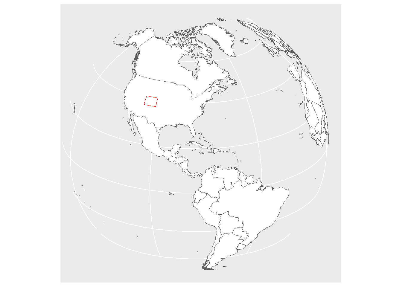
Colorado is a very interesting state with a simple boundary. The sourthern edge is 37 degrees latitude. The northern edge is 41 degrees north latitude. The eastern edge is 102 degrees, 02 minutes, 48 seconds west longitude. The western edge is 109 degrees, 02 minutes, 48 seconds west longitude.
You can calculate the length of each of these boundaries with a bit of simple math. The radius of the earth is 6,378 kilometers. So the circumference is
r <- 6378
2*pi*r
[1] 40074.16Each degree of latitude is
2*pi*r/360[1] 111.3171So the four degrees that you would have to travel to get from the southern border (37 degrees) to the northern border (41 degrees) is
2*pi*r*4/360[1] 445.2684The distance from the east to the west border is tricky. At the equator a degree of distance is 111.3 meters, but as you move away from the equator, the lines of latitude converge so a degree of longitude shrinks. A simple bit of geometry can show you that a single degree of longitude at 37 degrees is
2*pi*r*cos(37*pi/180)/360[1] 88.90179but at 41 degrees, it is
2*pi*r*cos(41*pi/180)/360[1] 84.01208That means that the 9 degrees that you travel from the eastern border to the western border is
2*pi*r*cos(37*pi/180)*9/360[1] 800.1161at 37 degrees, but only
2*pi*r*cos(41*pi/180)*9/360[1] 756.1087So the northern border of Colorado is shorter than the southern border.
And all this time you thought Colorado was a rectangle! It’s not. It is not a trapezoid either. It exists on a three dimensional globe and is more complex than any two dimensional geometric object can represent.
You need to make a projection any time you try to represent a three dimensional object like the state of Colorado on a two dimensional medium like a computer screen or a sheet of paper. Here is the Lambert projection.
projection_string <- "+proj=laea +lon_0=-105.5 +lat_0=39 +datum=WGS84 +no_defs"
co %>%
  ggplot() +
  geom_sf(color="red", fill="white") +
  coord_sf(crs=projection_string)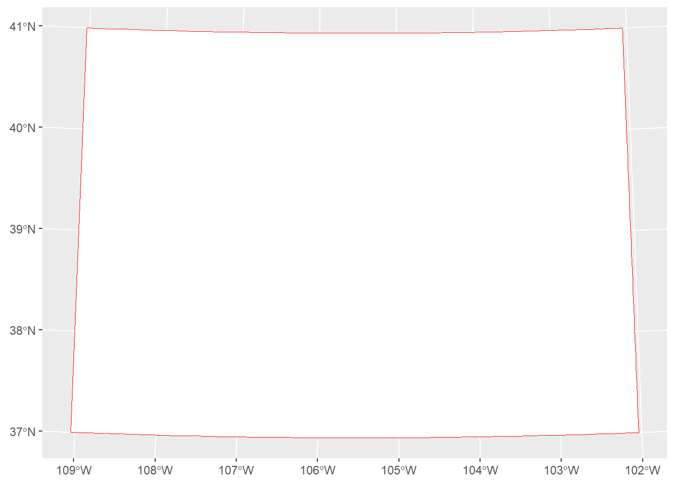
Notice that it has to warp some of the straight edge boundaries in order to keep the distances correct at the northern and southern borders.
Plotting the entire continent of North America shows even more warping. Notice how the state of Alaska has been twisted almost 45 degrees to accomodate. The island of Greenland is also twisted but in the opposite direction.
The distortions of the Lambert projection are more extreme when you are trying to fit large distances into a single map. The distortions become most noticeable at the edges. There is almost no distortion near the center.
projection_string <- "+proj=laea +lon_0=-105.5 +lat_0=39 +datum=WGS84 +no_defs"
countries %>%
  filter(continent=="North America") %>%
  ggplot() +
  geom_sf(color="red", fill="white") +
  coord_sf(crs=projection_string)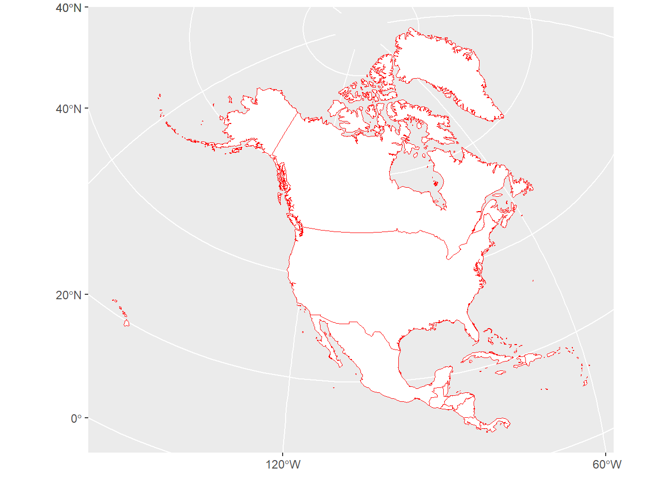
The most common projection is the Mercator projection. Here is the Mercator projection for the state of Colorado.
projection_string <- "+proj=merc +lon_0=0 +datum=WGS84 +no_defs"
co %>%
  ggplot() +
  geom_sf(color="red", fill="white") +
  coord_sf(crs=projection_string)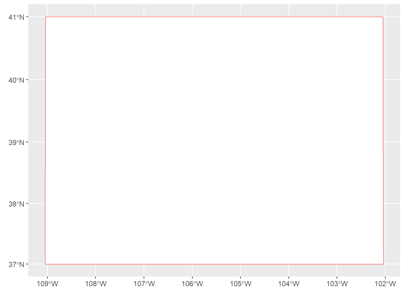
No warping of the boundaries but the lengths of the northern and southern borders are displayed incorrectly as having the same length. Not only are distances distorted, but areas as well. That becomes more obvious when you look at the entire continent.
projection_string <- "+proj=merc +lon_0=-105.5 +datum=WGS84 +no_defs"
countries %>%
  filter(continent=="North America") %>%
  ggplot() +
  geom_sf(color="red", fill="white") +
  coord_sf(crs=projection_string)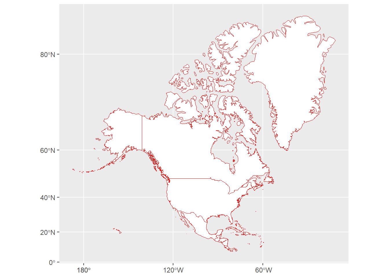
Notice how Alaska has grown to more than half the size of the rest of the United States. Alaska is big, but not that big! Also Greenland has expanded to monstrous proportions. The Mercator projection is simple, but it has a lot of distortions at the higher latitudes.
But notice how the eastern border of the state of Alaska is perfectly vertical, representing a true north/south orientation.
No projection system is perfect, and you should try different approaches to see what works best for your situation.