library(broom)
library(dplyr)
library(ggplot2)
library(foreign)
library(magrittr)
library(pscl)There are a broad range of diagnostic methods (mostly graphical) that can help you decide from among a dizzying array of alternative models for count data. The most important consideration is to start at the shallow end of the pool with the simplest approaches. Don’t jump in at the deep end and try something really complex before you’ve had the chance to look at simpler models, even if you know they are overly simplistic.
The dataset used in this example
Francis Huang has a nice web page showing two datasets and how to analyze them using the Poisson regression model as well as several more sophisticated models. The first data set is available for anyone to download. The link I originally used no longer works.
fn <- "http://faculty.missouri.edu/huangf/data/poisson/articles.csv"
articles <- read.csv(fn)
head(articles)
Here is a different link for the same file, used at German Rodriguez’s website. I’ve placed a copy on my website in case this link breaks. Also, this dataset is available with the pscl library of R under the name, bioChemists.
fn <- "http://www.pmean.com/00files/couart2.dta"
articles <- read.dta(fn)
head(articles)
art fem mar kid5 phd ment
1 0 Men Married 0 2.52 7
2 0 Women Single 0 2.05 6
3 0 Women Single 0 3.75 6
4 0 Men Married 1 1.18 3
5 0 Women Single 0 3.75 26
6 0 Women Married 2 3.59 2The variables are + gender (fem), + marital status (mar), + number of children (kid5), + prestige of graduate program (phd), + the number of articles published by the individual’s mentor (ment) + the number of articles published by the scientist (art: the outcome).
Histogram of outcome variable
Look at the possible values for your outcome variable, which is usually a count. If you have rate data, do a histogram both for counts and rates.
ggplot(articles, aes(art)) +
  geom_histogram(binwidth=1, color="black", fill="white")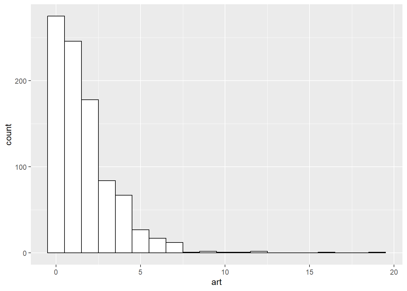
Compare this to a bar chart of Poisson probabilities. The outcome variable from a Poisson regression model does not need to follow a single simple Poisson set of probabilities. It is more likely a mixture of different Poisson variables depending on the covariate pattern. Nevertheless, it can’t hurt to look at the Poisson probabilities, as long as you don’t get too concerned about discrepancies between the actual data and the Poisson probabilities.
data.frame(x=0:max(articles$art)) %>%
  mutate(p=dpois(x, lambda=mean(articles$art))) %>%
  ggplot(aes(factor(x), p)) +
    geom_col(color="black", fill="white")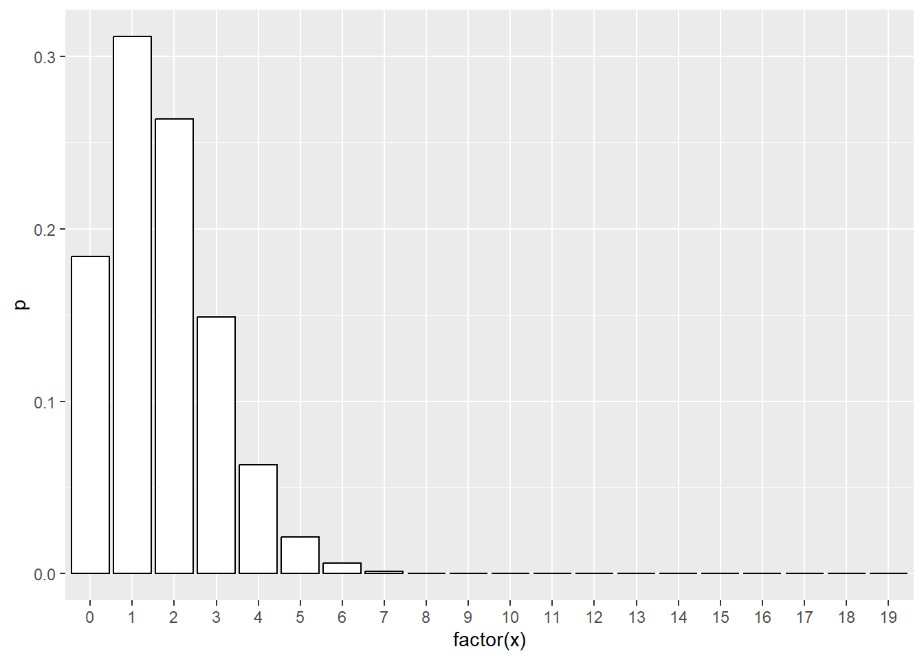
Here there seems to be a disparity at zero, which may (or may not) indicate the need for a zero-inflated model.
Descriptive statistics on indepdent variables
It helps to know the general descriptive statistics (means, standard deviations, percentages) for each of the independent variables.
articles %>%
  group_by(fem) %>%
  summarize(n=n())
# A tibble: 2 × 2
fem n
<fct> <int>
1 Men 494
2 Women 421quantile(articles$ment) 0% 25% 50% 75% 100%
0 3 6 12 77 quantile(articles$phd) 0% 25% 50% 75% 100%
0.755 2.260 3.150 3.920 4.620 articles %>%
group_by(mar) %>%
summarize(n=n())# A tibble: 2 × 2
mar n
<fct> <int>
1 Single 309
2 Married 606```{rglm-diagnostics-10
articles %>% group_by(kid5) %>% summarize(n=n())
The wide ranges for ment and phd may make it difficult to interpret. A simple approach is to scale them to the interval 0 to 1.


::: {.cell}

```{.r .cell-code}
articles %>%
  mutate(ment=(ment-min(ment))/(max(ment)-min(ment))) %>%
  mutate(phd=(phd-min(phd))/(max(phd)-min(phd))) -> articles_scaled
:::
Bivariate plots
Although you are going to fit multiple independent variables, it does not hurt to look at the bivariate relationships first. A variable that looks important from a bivariate perspective, may be unimportant from the multivariate perspective and vice versa. So don’t read too much into these plots. It is intended to get you familiar with trends and patterns that might (or might not) show up in more complex models.
Use boxplots when the independent variable is categorical and scatterplots when the independent variable is continuous.
ggplot(articles, aes(factor(fem), art)) +
  geom_boxplot()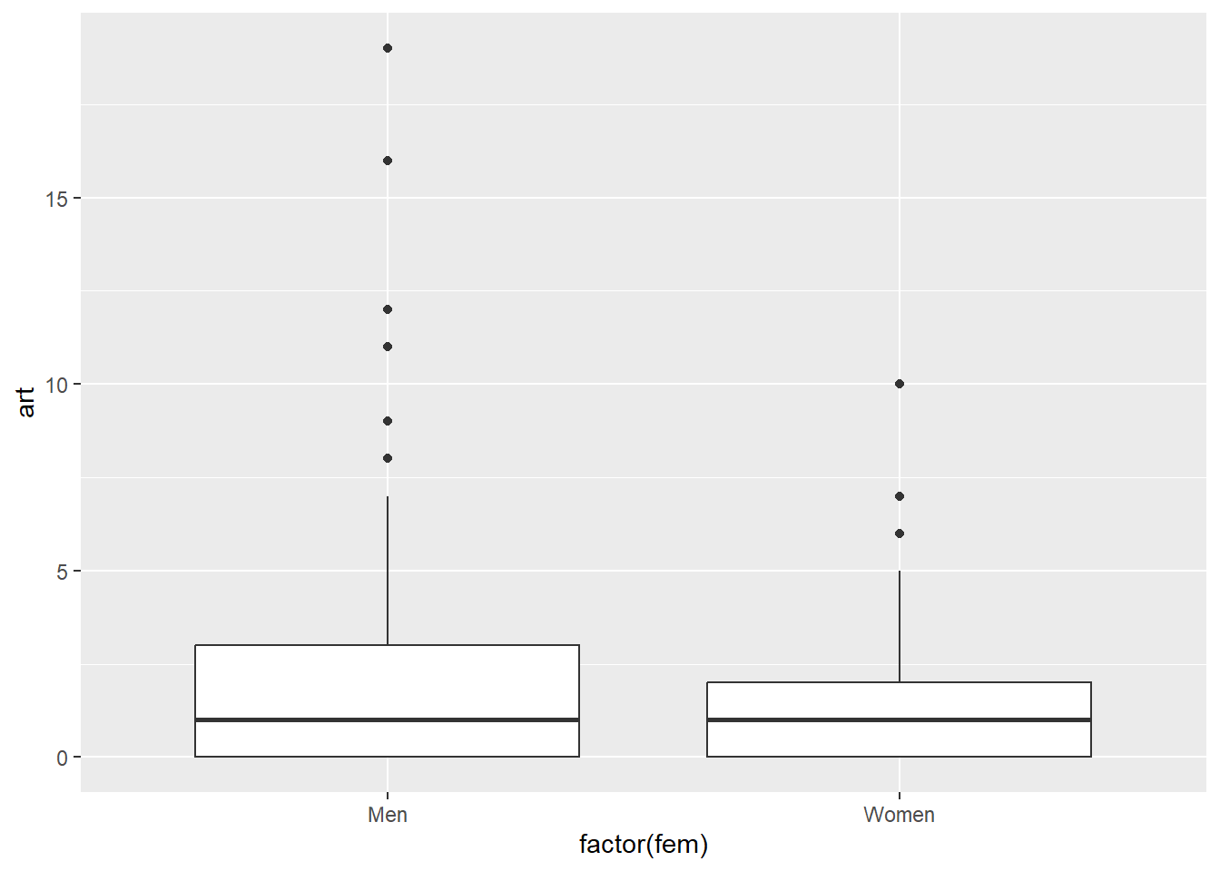
ggplot(articles, aes(ment, art)) +
  geom_point() +
  geom_smooth()
`geom_smooth()` using method = 'loess' and formula = 'y ~ x'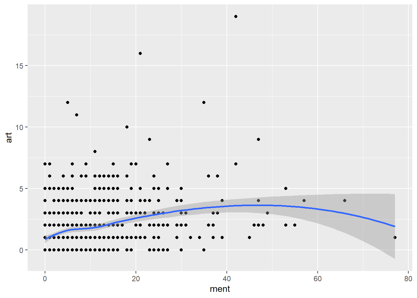
ggplot(articles, aes(phd, art)) +
  geom_point() +
  geom_smooth()
`geom_smooth()` using method = 'loess' and formula = 'y ~ x'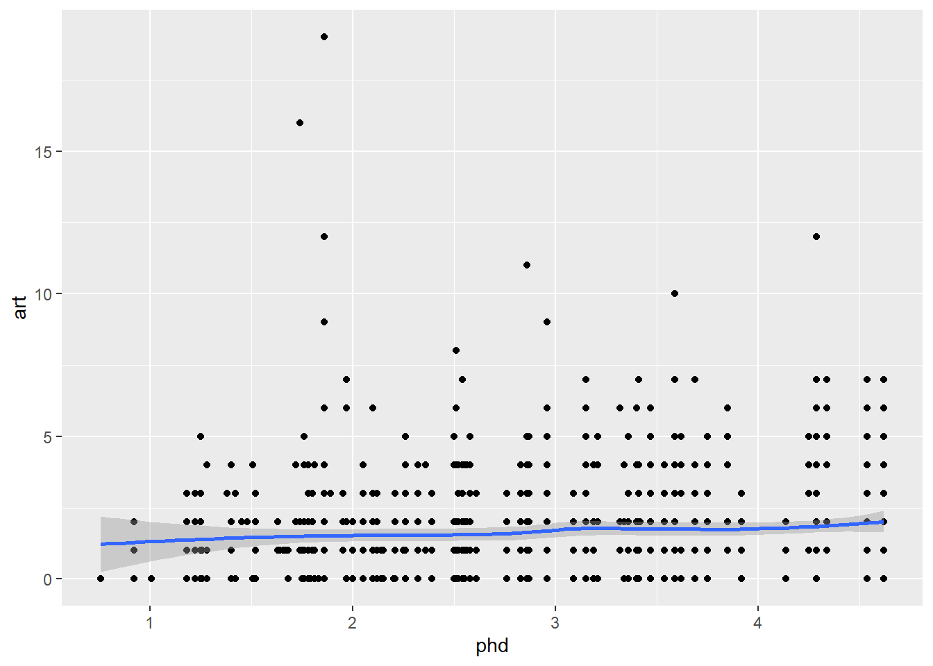
ggplot(articles, aes(factor(mar), art)) +
  geom_boxplot()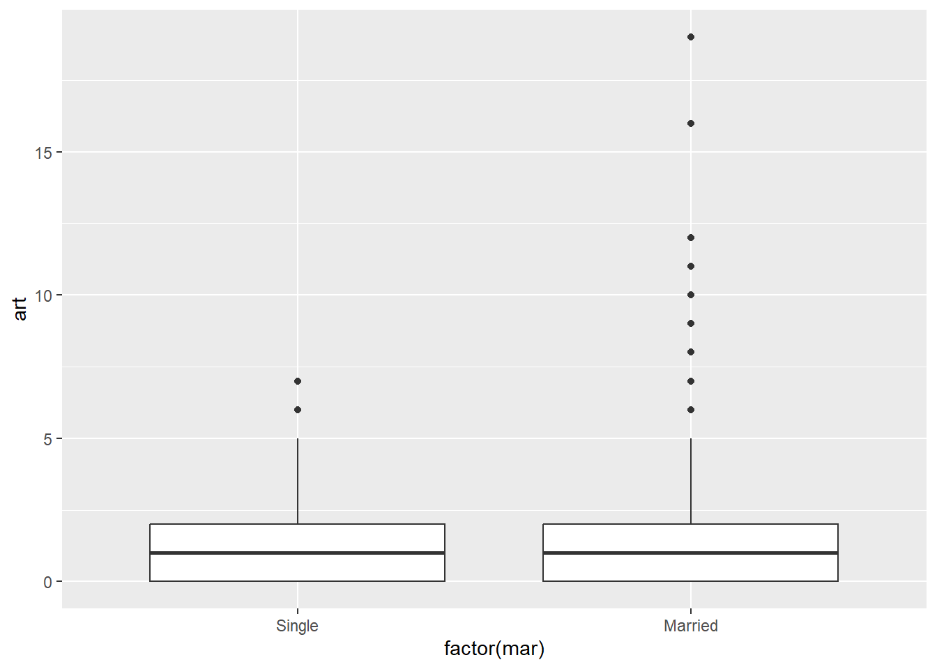
ggplot(articles, aes(factor(kid5), art)) +
  geom_boxplot()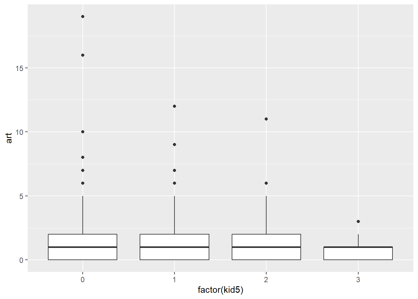
There aren’t any huge trends here. It looks like there might not be much going on here at all. If there are differences, they seem to show up in the values above the 75th percentile.
The one cause for early concern is that the effect of ment seems to level off after a certain point.
Fit simple models first
pois_fem <- glm(art ~ fem, family=poisson, data = articles_scaled)
summary(pois_fem)
Call:
glm(formula = art ~ fem, family = poisson, data = articles_scaled)

Coefficients:
            Estimate Std. Error z value Pr(>|z|)
(Intercept)  0.63265    0.03279  19.293  < 2e-16 ***
femWomen    -0.24718    0.05187  -4.765 1.89e-06 ***
---
Signif. codes:  0 '***' 0.001 '**' 0.01 '*' 0.05 '.' 0.1 ' ' 1

(Dispersion parameter for poisson family taken to be 1)

    Null deviance: 1817.4  on 914  degrees of freedom
Residual deviance: 1794.4  on 913  degrees of freedom
AIC: 3466.1

Number of Fisher Scoring iterations: 5
pois_ment <- glm(art ~ ment, family=poisson, data = articles_scaled)
summary(pois_ment)
Call:
glm(formula = art ~ ment, family = poisson, data = articles_scaled)

Coefficients:
            Estimate Std. Error z value Pr(>|z|)
(Intercept)  0.25991    0.03436   7.564 3.91e-14 ***
ment         2.00584    0.14764  13.586  < 2e-16 ***
---
Signif. codes:  0 '***' 0.001 '**' 0.01 '*' 0.05 '.' 0.1 ' ' 1

(Dispersion parameter for poisson family taken to be 1)

    Null deviance: 1817.4  on 914  degrees of freedom
Residual deviance: 1669.5  on 913  degrees of freedom
AIC: 3341.3

Number of Fisher Scoring iterations: 5
pois_phd <- glm(art ~ phd, family=poisson, data = articles_scaled)
summary(pois_phd)
Call:
glm(formula = art ~ phd, family = poisson, data = articles_scaled)

Coefficients:
            Estimate Std. Error z value Pr(>|z|)
(Intercept)  0.32259    0.06813   4.735 2.19e-06 ***
phd          0.32976    0.10053   3.280  0.00104 **
---
Signif. codes:  0 '***' 0.001 '**' 0.01 '*' 0.05 '.' 0.1 ' ' 1

(Dispersion parameter for poisson family taken to be 1)

    Null deviance: 1817.4  on 914  degrees of freedom
Residual deviance: 1806.6  on 913  degrees of freedom
AIC: 3478.3

Number of Fisher Scoring iterations: 5
pois_mar <- glm(art ~ mar, family=poisson, data = articles_scaled)
summary(pois_mar)
Call:
glm(formula = art ~ mar, family = poisson, data = articles_scaled)

Coefficients:
            Estimate Std. Error z value Pr(>|z|)
(Intercept)  0.46514    0.04508  10.317   <2e-16 ***
marMarried   0.09117    0.05458   1.671   0.0948 .
---
Signif. codes:  0 '***' 0.001 '**' 0.01 '*' 0.05 '.' 0.1 ' ' 1

(Dispersion parameter for poisson family taken to be 1)

    Null deviance: 1817.4  on 914  degrees of freedom
Residual deviance: 1814.6  on 913  degrees of freedom
AIC: 3486.3

Number of Fisher Scoring iterations: 5
pois_kid5 <- glm(art ~ kid5, family=poisson, data = articles_scaled)
summary(pois_kid5)
Call:
glm(formula = art ~ kid5, family = poisson, data = articles_scaled)

Coefficients:
            Estimate Std. Error z value Pr(>|z|)
(Intercept)  0.55960    0.02988  18.728   <2e-16 ***
kid5        -0.06978    0.03450  -2.023   0.0431 *
---
Signif. codes:  0 '***' 0.001 '**' 0.01 '*' 0.05 '.' 0.1 ' ' 1

(Dispersion parameter for poisson family taken to be 1)

    Null deviance: 1817.4  on 914  degrees of freedom
Residual deviance: 1813.2  on 913  degrees of freedom
AIC: 3485

Number of Fisher Scoring iterations: 5
For all of these models, the deviance is much greater than the degrees of freedom, indicating a poor fit. This could be failure to include all the variables in a multivariate sense or a problem with the underlying Poisson model.
Don’t put too much stock in the p-values just yet, but several of them are small. This may change when we look at the independent variables in combination.
Fit graually more complex models
pois_all_ivs <- glm(art ~ fem + ment + phd + mar + kid5, family=poisson, data = articles_scaled)
summary(pois_all_ivs)
Call:
glm(formula = art ~ fem + ment + phd + mar + kid5, family = poisson,
    data = articles_scaled)

Coefficients:
            Estimate Std. Error z value Pr(>|z|)
(Intercept)  0.31430    0.08758   3.589 0.000332 ***
femWomen    -0.22459    0.05461  -4.112 3.92e-05 ***
ment         1.96679    0.15447  12.733  < 2e-16 ***
phd          0.04956    0.10202   0.486 0.627139
marMarried   0.15524    0.06137   2.529 0.011424 *
kid5        -0.18488    0.04013  -4.607 4.08e-06 ***
---
Signif. codes:  0 '***' 0.001 '**' 0.01 '*' 0.05 '.' 0.1 ' ' 1

(Dispersion parameter for poisson family taken to be 1)

    Null deviance: 1817.4  on 914  degrees of freedom
Residual deviance: 1634.4  on 909  degrees of freedom
AIC: 3314.1

Number of Fisher Scoring iterations: 5tidy(pois_fem) %>%
bind_rows(tidy(pois_ment)) %>%
bind_rows(tidy(pois_phd)) %>%
bind_rows(tidy(pois_mar)) %>%
bind_rows(tidy(pois_kid5)) %>%
filter(term != "(Intercept)") %>%
mutate(unadjusted_rate_ratio=round(exp(estimate), 2)) %>%
select(term, unadjusted_rate_ratio) -> pois_crude
tidy(pois_all_ivs) %>%
filter(term != "(Intercept)") %>%
mutate(adjusted_rate_ratio=round(exp(estimate), 2)) %>%
select(term, adjusted_rate_ratio) -> pois_adjust
pois_crude %>%
full_join(pois_adjust)Joining with `by = join_by(term)`# A tibble: 5 × 3
term unadjusted_rate_ratio adjusted_rate_ratio
<chr> <dbl> <dbl>
1 femWomen 0.78 0.8
2 ment 7.43 7.15
3 phd 1.39 1.05
4 marMarried 1.1 1.17
5 kid5 0.93 0.83Examine residuals
A good general plot is fitted (predicted) values versus residuals. Since the fitted value is a composite of all the independent variables, it is likely to show unusual behavior if there are issues involving any of the independent variables.
An ideal pattern would be a random scatter of points spread across all regions of the graph. A curvilinear pattern (e.g., high in the middle, low at either extreme) or a fanning out pattern (e.g., more variation on the right side of the graph than the left) is indication that there are unusual features in the data that are not fully captured by the current model.
r_pois <- augment(pois_all_ivs, articles_scaled, type.predict="response", type.residuals="deviance")
ggplot(r_pois, aes(.fitted, .resid)) +
  geom_point() +
  geom_smooth()
`geom_smooth()` using method = 'loess' and formula = 'y ~ x'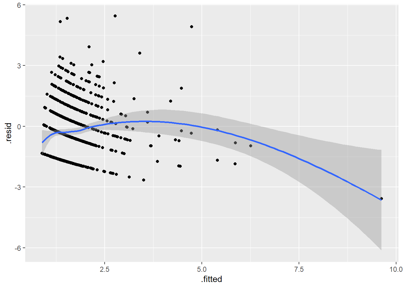
Clearly there is something unusual going on with the largest fitted value.
r_pois %>%
  filter(.fitted > 7) %>%
  data.frame
art fem mar kid5 phd ment .fitted .resid .hat .sigma
1 1 Men Married 1 0.2652005 1 9.627207 -3.567244 0.1993306 1.33509
.cooksd .std.resid
1 0.4006419 -3.986632This appears to be the subject where the scaled value for ment equals 1. In other words, the highest possible value for ment.
You should also plot the residuals versus every independent variable, although the plots versus binary independent variables are unlikely to show anything interesting.
ggplot(r_pois, aes(factor(fem), .resid)) +
  geom_boxplot()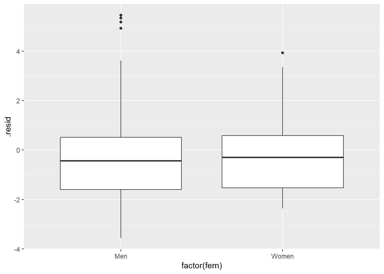
ggplot(r_pois, aes(ment, .resid)) +
  geom_point() +
  geom_smooth()
`geom_smooth()` using method = 'loess' and formula = 'y ~ x'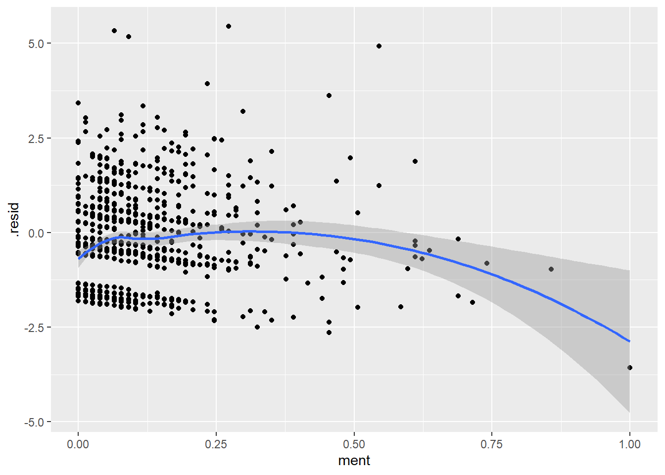
ggplot(r_pois, aes(phd, .resid)) +
  geom_point() +
  geom_smooth()
`geom_smooth()` using method = 'loess' and formula = 'y ~ x'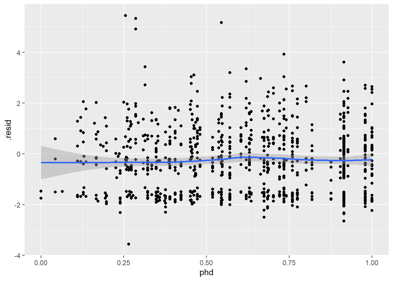
ggplot(r_pois, aes(factor(mar), .resid)) +
  geom_boxplot()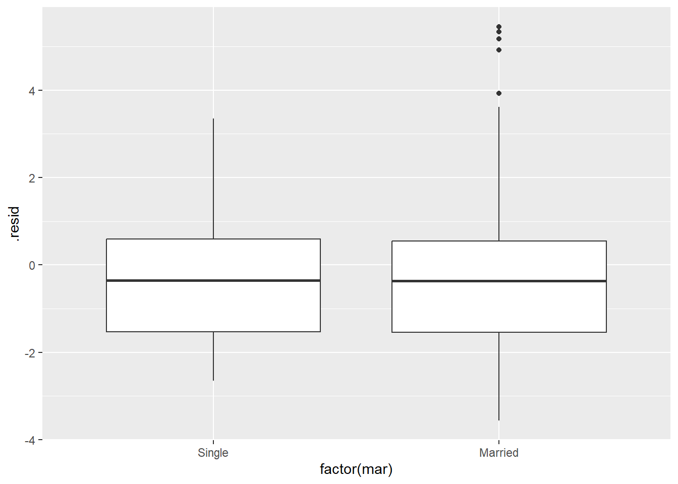
ggplot(r_pois, aes(factor(kid5), .resid)) +
  geom_boxplot()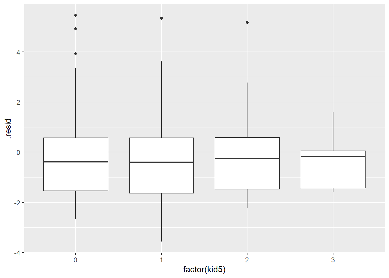
Perhaps, the value of a mentor is good only to a point and anything after offers no additional help. Let’s compute a new value for ment where any value above 40 is set equal to 40.
articles %>%
  mutate(ment=pmin(40, ment)) %>%
  mutate(ment=(ment-min(ment))/(max(ment)-min(ment))) %>%
  mutate(phd=(phd-min(phd))/(max(phd)-min(phd))) -> articles_rescaled
pois_rescaled <-
  glm(
    art ~ fem + ment + phd + mar + kid5,
      family=poisson,
        data = articles_rescaled)
r_rescaled <-
  augment(
    pois_rescaled,
      articles_rescaled,
        type.predict="response",
          type.residuals="deviance")
ggplot(r_rescaled, aes(.fitted, .resid)) +
  geom_point() +
  geom_smooth()
`geom_smooth()` using method = 'loess' and formula = 'y ~ x'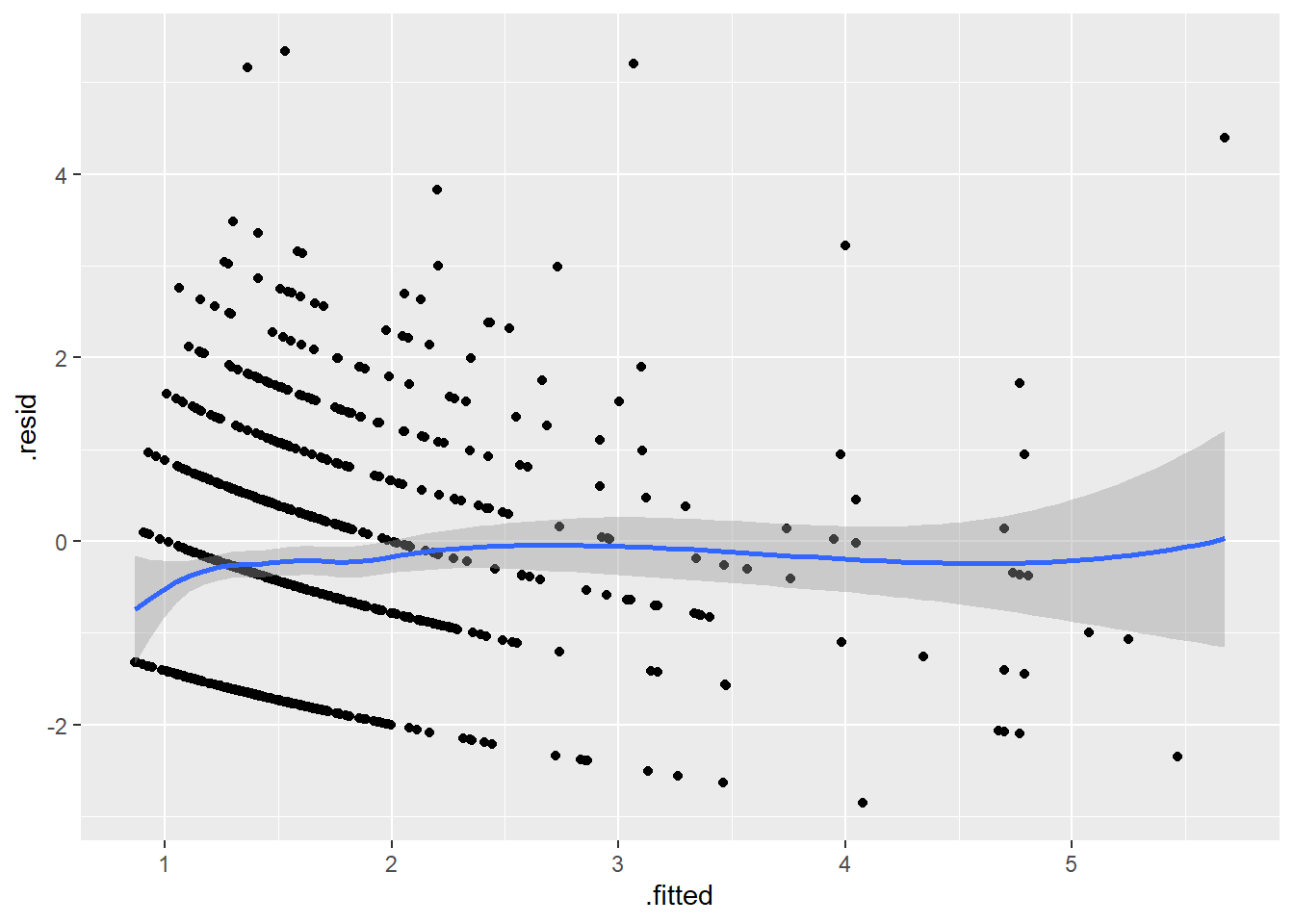
ggplot(r_rescaled, aes(ment, .resid)) +
  geom_point() +
  geom_smooth()
`geom_smooth()` using method = 'loess' and formula = 'y ~ x'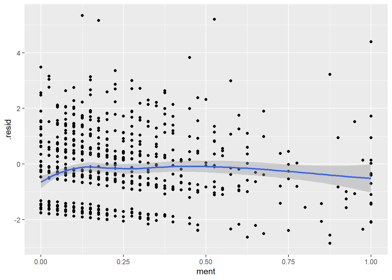
Negative binomial model
library(MASS)
Attaching package: 'MASS'The following object is masked from 'package:dplyr':
selectnb1 <- glm.nb(art ~ fem + ment + phd + mar + kid5, data = articles_rescaled)
summary(pois_rescaled)
Call:
glm(formula = art ~ fem + ment + phd + mar + kid5, family = poisson,
    data = articles_rescaled)

Coefficients:
            Estimate Std. Error z value Pr(>|z|)
(Intercept)  0.28876    0.08797   3.283  0.00103 **
femWomen    -0.22336    0.05453  -4.096  4.2e-05 ***
ment         1.29786    0.09771  13.283  < 2e-16 ***
phd         -0.02054    0.10361  -0.198  0.84284
marMarried   0.15519    0.06136   2.529  0.01143 *
kid5        -0.17383    0.03987  -4.360  1.3e-05 ***
---
Signif. codes:  0 '***' 0.001 '**' 0.01 '*' 0.05 '.' 0.1 ' ' 1

(Dispersion parameter for poisson family taken to be 1)

    Null deviance: 1817.4  on 914  degrees of freedom
Residual deviance: 1612.3  on 909  degrees of freedom
AIC: 3292.1

Number of Fisher Scoring iterations: 5summary(nb1)
Call:
glm.nb(formula = art ~ fem + ment + phd + mar + kid5, data = articles_rescaled,
    init.theta = 2.345482748, link = log)

Coefficients:
            Estimate Std. Error z value Pr(>|z|)
(Intercept)  0.24464    0.11622   2.105  0.03530 *
femWomen    -0.21377    0.07215  -2.963  0.00305 **
ment         1.34279    0.14614   9.188  < 2e-16 ***
phd          0.02888    0.13882   0.208  0.83517
marMarried   0.15054    0.08156   1.846  0.06494 .
kid5        -0.17066    0.05240  -3.257  0.00113 **
---
Signif. codes:  0 '***' 0.001 '**' 0.01 '*' 0.05 '.' 0.1 ' ' 1

(Dispersion parameter for Negative Binomial(2.3455) family taken to be 1)

    Null deviance: 1122.1  on 914  degrees of freedom
Residual deviance: 1008.1  on 909  degrees of freedom
AIC: 3128.3

Number of Fisher Scoring iterations: 1

              Theta:  2.345
          Std. Err.:  0.289

 2 x log-likelihood:  -3114.311
Zero inflated model
zip1 <-
  zeroinfl(
    art ~ fem + ment + phd + mar + kid5 |
      1,
        dist="poisson",
          data = articles_rescaled)
summary(zip1)
Call:
zeroinfl(formula = art ~ fem + ment + phd + mar + kid5 | 1, data = articles_rescaled,
    dist = "poisson")

Pearson residuals:
    Min      1Q  Median      3Q     Max
-1.4952 -0.9862 -0.2940  0.5601  7.3463

Count model coefficients (poisson with log link):
            Estimate Std. Error z value Pr(>|z|)
(Intercept)  0.52080    0.09770   5.331 9.79e-08 ***
femWomen    -0.23166    0.05824  -3.978 6.96e-05 ***
ment         1.13674    0.10570  10.754  < 2e-16 ***
phd         -0.05874    0.11145  -0.527 0.598140
marMarried   0.13225    0.06574   2.012 0.044239 *
kid5        -0.16129    0.04285  -3.765 0.000167 ***

Zero-inflation model coefficients (binomial with logit link):
            Estimate Std. Error z value Pr(>|z|)
(Intercept)  -1.7435     0.1639  -10.63   <2e-16 ***
---
Signif. codes:  0 '***' 0.001 '**' 0.01 '*' 0.05 '.' 0.1 ' ' 1

Number of iterations in BFGS optimization: 13
Log-likelihood: -1611 on 7 Df
zip2 <-
zeroinfl(
art ~ fem + ment + phd + mar + kid5 |
fem + ment + phd + mar + kid5,
dist="poisson",
data = articles_rescaled)
summary(zip2)
Call:
zeroinfl(formula = art ~ fem + ment + phd + mar + kid5 | fem + ment +
    phd + mar + kid5, data = articles_rescaled, dist = "poisson")

Pearson residuals:
    Min      1Q  Median      3Q     Max
-1.9307 -0.8803 -0.2634  0.5320  7.0179

Count model coefficients (poisson with log link):
            Estimate Std. Error z value Pr(>|z|)
(Intercept)  0.62199    0.10366   6.000 1.97e-09 ***
femWomen    -0.21558    0.06390  -3.374 0.000741 ***
ment         0.96293    0.11653   8.263  < 2e-16 ***
phd         -0.09387    0.12331  -0.761 0.446502
marMarried   0.10351    0.07184   1.441 0.149635
kid5        -0.13632    0.04756  -2.866 0.004156 **

Zero-inflation model coefficients (binomial with logit link):
            Estimate Std. Error z value Pr(>|z|)
(Intercept) -0.61145    0.43313  -1.412  0.15804
femWomen     0.06827    0.28564   0.239  0.81109
ment        -4.03326    1.45417  -2.774  0.00554 **
phd         -0.21522    0.56689  -0.380  0.70421
marMarried  -0.34733    0.32230  -1.078  0.28118
kid5         0.22108    0.19709   1.122  0.26198
---
Signif. codes:  0 '***' 0.001 '**' 0.01 '*' 0.05 '.' 0.1 ' ' 1

Number of iterations in BFGS optimization: 21
Log-likelihood: -1599 on 12 Df
zip3 <-
zeroinfl(
art ~ fem + ment + phd + mar + kid5 |
ment,
dist="poisson",
data = articles_rescaled)
summary(zip3)
Call:
zeroinfl(formula = art ~ fem + ment + phd + mar + kid5 | ment, data = articles_rescaled,
    dist = "poisson")

Pearson residuals:
    Min      1Q  Median      3Q     Max
-1.9318 -0.8877 -0.2517  0.5310  7.0536

Count model coefficients (poisson with log link):
            Estimate Std. Error z value Pr(>|z|)
(Intercept)  0.59978    0.09752   6.150 7.74e-10 ***
femWomen    -0.22165    0.05874  -3.774 0.000161 ***
ment         0.96217    0.11360   8.470  < 2e-16 ***
phd         -0.07773    0.11213  -0.693 0.488213
marMarried   0.13383    0.06630   2.018 0.043546 *
kid5        -0.15649    0.04324  -3.619 0.000295 ***

Zero-inflation model coefficients (binomial with logit link):
            Estimate Std. Error z value Pr(>|z|)
(Intercept)  -0.8236     0.2141  -3.847  0.00012 ***
ment         -4.1956     1.3978  -3.002  0.00269 **
---
Signif. codes:  0 '***' 0.001 '**' 0.01 '*' 0.05 '.' 0.1 ' ' 1

Number of iterations in BFGS optimization: 14
Log-likelihood: -1600 on 8 Df
zinb <-
zeroinfl(
art ~ fem + ment + phd + mar + kid5 |
ment,
dist="negbin",
data = articles_rescaled)
summary(zinb)
Call:
zeroinfl(formula = art ~ fem + ment + phd + mar + kid5 | ment, data = articles_rescaled,
    dist = "negbin")

Pearson residuals:
    Min      1Q  Median      3Q     Max
-1.2732 -0.7706 -0.2525  0.4796  6.4457

Count model coefficients (negbin with log link):
            Estimate Std. Error z value Pr(>|z|)
(Intercept)  0.37538    0.12149   3.090  0.00200 **
femWomen    -0.21021    0.07162  -2.935  0.00333 **
ment         1.14750    0.15473   7.416 1.21e-13 ***
phd         -0.01688    0.13731  -0.123  0.90214
marMarried   0.14006    0.08088   1.732  0.08331 .
kid5        -0.16263    0.05218  -3.117  0.00183 **
Log(theta)   1.01830    0.14352   7.095 1.29e-12 ***

Zero-inflation model coefficients (binomial with logit link):
            Estimate Std. Error z value Pr(>|z|)
(Intercept)  -0.8630     0.3706  -2.329   0.0199 *
ment        -25.3534    10.5777  -2.397   0.0165 *
---
Signif. codes:  0 '***' 0.001 '**' 0.01 '*' 0.05 '.' 0.1 ' ' 1

Theta = 2.7685
Number of iterations in BFGS optimization: 36
Log-likelihood: -1550 on 9 Df
Comparing competing models
The AIC statistic is useful for comparing models, but it is not produced automatically for negative binomial regression or the zero-inflated models. It requires you to pull the individual components from the
save.image(file="glm_diagnostics.RData")An earlier version of this page was published on new.pmean.com.