News: Sign up for "The Monthly Mean," the newsletter that dares to call itself average, www.pmean.com/news.
This page has moved to a new website
.| P.Mean: What are wavelets? (created 2014-03-01).
News: Sign up for "The Monthly Mean," the newsletter that dares to call itself average, www.pmean.com/news. |
Wavelets represent a method to decompose a signal or an image. It represents an alternative to the Fourier decomposition. It is useful in image compression, edge analysis and flexible de-noising of even complicated discontinuous functions. Although there are adaptations to more complex settings, wavelets work best when analyzing a signal that is sampled at evenly spaced time points.
To understand wavelets well, you need to refresh yourself on how the Fourier decomposition really works. Think about Fourier as a way to travel to Trigland, the land of sines and cosines.
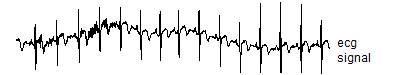
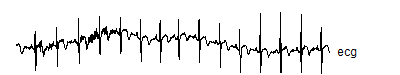
There is data set with the wavelets package in R called "ecg" that represents 2048 evenly spaced values from a typical electrocardiogram. Here's the code to get and graph that signal
> library("rwt")

  > library("wavelets")

   > data(ecg)

    > head(ecg)

     [1] -0.104773 -0.093136 -0.081500 -0.116409 -0.081500 -0.116409

     > tail(ecg)

      [1] -0.430591 -0.442227 -0.477136 -0.442227 -0.477136 -0.477136

      > graph.axis("wave00.png")

       null device

1

> graph.single("wave01.png",ecg,"ecg\nsignal",c(-1.5,1.5))

 null device

1
The head and tail function show the first few and the last few values for the signal. The graph looks like
![]()
You can ignore the units of the signal itself, as they are arbitrary (at least for this application), but the minimum value is -1.48 and the maximum is 1.44. You compute the Fourier decomposition using the fft command, which is part of the base R package. The letters stand for "fast fourier transform".
> ft.ecg <- fft(ecg)/2048

  > head(ft.ecg)

   [1] -0.040859772+0.000000000i -0.144005054-0.128781054i

   [3] -0.004311727+0.007706751i  0.023643179+0.046245122i

   [5]  0.004964307-0.026597976i -0.010241779+0.017355456i

   > tail(ft.ecg)

    [1]  0.010344229+0.000402821i -0.010241779-0.017355456i

    [3]  0.004964307+0.026597976i  0.023643179-0.046245122i

    [5] -0.004311727-0.007706751i -0.144005054+0.128781054i

    > ift.ecg <- fft(ft.ecg,inverse=TRUE)

     > head(ift.ecg)

      [1] -0.104773-0i -0.093136+0i -0.081500-0i -0.116409+0i -0.081500-0i

      [6] -0.116409+0i

      > tail(ift.ecg)

       [1] -0.430591+0i -0.442227+0i -0.477136+0i -0.442227-0i -0.477136-0i

       [6] -0.477136-0i
The object ft.ecg contains the Fourier decomposition, and ift.ecg is the inverse of the decomposition. You need to scale the Fourier decomposition by the number of data points (2,048). The inverse gets the original signal (-0.104773, -0.081500, -0.116409,...) except that there is a "+0i" or "-0i" tacked on to the end.
The complex numbers in the Fourier decomposition are a short-hand for the mix of sines and cosines. The first number has only a real component and no imaginary component. The real component represent the mean of the entire signal.
> comp(mean(ecg),Re(ft.ecg[1]),"ft[1]")

ft[1]

By hand -0.04085977

Using R -0.04085977
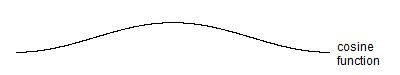
For the remaining numbers, the real part represents the cosine function and the imaginary part represents the sine function. So -0.144005054-0.128781054i represents -0.144005054*cos(2*pi*t) and -0.128781054*sin(2*pi*t). The following code shows the graph of the cosine function, the sine function and the sum.
> t.unit <- (1:2048)/2048

  > cos1 <- +Re(ft.ecg[2])*cos(2*pi*t.unit)

   > graph.single("wave02.png",cos1,"cosine\nfunction",c(-0.35,0.35))

    null device

1

> sin1 <- -Im(ft.ecg[2])*sin(2*pi*t.unit)

 > graph.single("wave03.png",sin1,"sine\nfunction",c(-0.35,0.35))

  null device

1

> sum1 <- cos1+sin1

 > graph.single("wave04.png",sum1,"Sum of\nsine and\ncosine",c(-0.35,0.35))

  null device

1
Here's the first graph.
![]()
The graph of the cosine function shows a peak halfway through (1024) and a trough at the end (or equivalently at the beginning). This is actually flipped around from the normal cosine function, but recall that the multiplier front of the cosine function is negative.
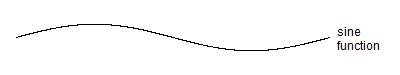
![]()
The graph of the sine function shows a peak at 1/4 of the the way through (512) and a trough 3/4 of the way through (1536).
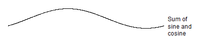
![]()
The sum shows the peak for the sum that is somewhere between the peaks of the sine and cosine functions. It's actually slightly closer to the peak of the cosine function, but not by much. The trough is also between the two troughs. The relative weights given to the sine and cosine functions and the positive or negative values associated with these weights will control where the peak and trough occur for the sum. In other words, you can control the phase of the curve.
If you are familiar with the arctangent function, you can compute the location of peak/trough. The Mod function will tell you the amplitude.
> ft.ratio <- -Im(ft.ecg[2])/Re(ft.ecg[2])

  > comp(round(2048*(atan(ft.ratio)+pi)/(2*pi)),which(sum1==max(sum1)),"Peak")

Peak

By hand  786

Using R  786

> comp(Mod(ft.ecg[2]),max(sum1),"Amplitude")

Amplitude

By hand 0.1931891

Using R 0.1931890
Now this was a lot of work to decode the second component of the Fourier decomposition. You might forget to scale by the length of the signal. You could reverse the sines and cosines. Yu might compute the sines and cosines on a range from -pi to pi instead of from 0 to 2pi. You might leave out an important minus sign. Trust me, I did all these things.
There's a faster and more convenient way. Let the computer do the work for you. Take the Fourier decomposition, zero out everything except the second component, and then invert the decomposition. This allows you to graph the second component directly.
> ft.comp2 <- rep(0,length(ft.ecg))

  > ft.comp2[2] <- ft.ecg[2]

   > comp2 <- Re(fft(ft.comp2,inverse=TRUE))

    > mx.2 <- max(comp2)

     > graph.single("wave05.png",comp2,"Second\nFourier\ncomponent",c(-0.35,0.35))

      null device

1
This is the graph
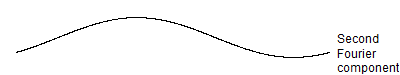
![]()
You can use the same method to show the shape of the third Fourier component.
> ft.comp3 <- rep(0,length(ft.ecg))

  > ft.comp3[3] <- ft.ecg[3]

   > comp3 <- Re(fft(ft.comp3,inverse=TRUE))

    > mx.3 <- max(comp3)

     > graph.single("wave06.png",comp3,"Third\nFourier\ncomponent",1.8*mx.3*c(-1,1))

      null device

1
Here is the graph
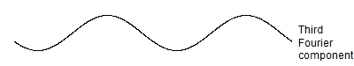
![]()
This component has a higher frequency, with two peaks rather than one. Do the same for the fourth Fourier component
> ft.comp4 <- rep(0,length(ft.ecg))

   > ft.comp4[4] <- ft.ecg[4]

    > comp4 <- Re(fft(ft.comp4,inverse=TRUE))

     > mx.4 <- max(comp4)

      > graph.single("wave07.png",comp4,"Fourth\nFourier\ncomponent",1.8*mx.4*c(-1,1))

       null device

1
Here is the graph.
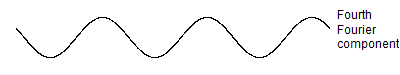
![]()
The fourth Fourier component has three peaks. The interesting thing is that the second and third and fourth Fourier components are orthogonal to one another. Actually, every Fourier component is orthogonal to every other Fourier component. Mathematical folks like "orthogonal" because it allows you to derive the mathematical properties of the decomposition with greater ease. For a practical person, what "orthogonal" means is that the information contained in one Fourier component does not "overlap" with that in any other Fourier component. It also means you can run the decomposition in any order (low frequency to high frequency, high frequency to low frequency, or even a haphazard frequency). Finally, orthogonality also preserves independence properties in certain settings.
The Fourier decomposition continues with components of higher and higher frequency. The following code computes the fiftieth component of the Fourier transform.
> ft.comp50 <- rep(0,length(ft.ecg))

  > ft.comp50[50] <- ft.ecg[50]

   > comp50 <- Re(fft(ft.comp50,inverse=TRUE))

    > mx.50 <- max(comp50)

     > mx <- 0.35*mx.50/mx.2

      > graph.single("wave08.png",comp50,"Fiftieth\nFourier\ncomponent",c(-mx,mx))

       null device

1
Here is the graph.
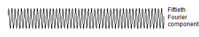
![]()
Here's the fiftieth Fourier component, and if you count carefully, you will get 49 peaks. Count them carefully. No, don't bother, I'll do it for you. Because that are packed so closely together, I will onlyshow you every third peak.
![]()
![]()
Now wavelets produce a deocomposition much like the Fourier decomposition but wavelets are different in one important way. Wavelets break the signal up into pieces and model signals within those pieces. The frequency of the wavelet signal is associated with the number of pieces. For high frequency wavelets, you break the signal up into a large number of pieces. For low frequency signals, you breah the signal up into fewer pieces.
There are at least two good R packages for wavelet docompositon, rwt and wavelets. Here's a brief overview of how rwt works.
> d4.rwt <- daubcqf(4)

  > d4.rwt

   $h.0

[1]  0.4829629  0.8365163  0.2241439 -0.1294095
$h.1

  [1]  0.1294095  0.2241439 -0.8365163  0.4829629
> wt.rwt <- mdwt(ecg,d4.rwt$h.0,L=9)

  > names(wt.rwt)

  [1] "y" "L"

  > head(wt.rwt$y)

  [,1]

  [1,]  0.797545

  [2,]  6.979219

  [3,] -2.933776

  [4,] -8.541192

  [5,]  4.087582

  [6,]  2.536293

  > tail(wt.rwt$y)

  [,1]

  [2043,]  0.003011394

  [2044,] -0.012342195

  [2045,]  0.001102199

  [2046,] -0.030707757

  [2047,] -0.007824638

  [2048,]  0.126029962

  > wt.rwt$L

  [1] 9

  > iwt.rwt <- midwt(wt.rwt$y,daub4$h.0,L=9)

  > names(iwt.rwt)

  [1] "x" "L"

  > head(iwt.rwt$x)

  [,1]

  [1,] -0.104773

  [2,] -0.093136

  [3,] -0.081500

  [4,] -0.116409

  [5,] -0.081500

  [6,] -0.116409

  > tail(iwt.rwt$x)

  [,1]

  [2043,] -0.430591

  [2044,] -0.442227

  [2045,] -0.477136

  [2046,] -0.442227

  [2047,] -0.477136

  [2048,] -0.477136

  > iwt.rwt$L

  [1] 9
With the rwt package, you choose the particular wavelet decomposition using the daubcqf function. The wavelet decomposition uses the mdwt function and the inverse of the wavelet decomposition uses the midwt decomposition. The rwt is fairly minimal with a family of Duabechies wavelts, but no alternatives (such as coiflets). Don't ask me what a coiflet is.
The wavelets package is more comprehensive, but also more complex.
> d4.wavelets <- wt.filter("d4")

  > d4.wavelets

   An object of class "wt.filter"

   Slot "L":

[1] 4
Slot "level":

  [1] 1
Slot "h":

  [1] -0.1294095 -0.2241439  0.8365163 -0.4829629
Slot "g":

  [1]  0.4829629  0.8365163  0.2241439 -0.1294095
Slot "wt.class":

  [1] "Daubechies"
Slot "wt.name":

  [1] "d4"
Slot "transform":

  [1] "dwt"
> wt.wavelets <- dwt(ecg,filter="d4")

  > slotNames(wt.wavelets)

  [1] "W"          "V"          "filter"     "level"      "n.boundary"

  [6] "boundary"   "series"     "class.X"    "attr.X"     "aligned"

  [11] "coe"

  > iwt.wavelets <- idwt(wt.wavelets)

  > head(iwt.wavelets)

  [1] -0.10477 -0.09314 -0.08150 -0.11641 -0.08150 -0.11641

  > tail(iwt.wavelets)

  [1] -0.43059 -0.44223 -0.47714 -0.44223 -0.47714 -0.47714
With the wavelets package, you choose the particular wavelet decomposition using the wt.filter function. The wavelet decomposition uses the dwt function and the inverse of the wavelet decomposition uses the idwt function. Notice that the wavelets package uses S4 objects.
I will use the rwt package for the rest of my examples. The S4 objects in wavelets are difficult to manipulate directly, and I could not get some of the hand calculations to match what this package computed. I'm sure the failure to get a match with my hand calculations is just because of my limitations.
I will also use the d4 or Daubechies 4 wavelet for these examples. Ingird Daubechies is one of the pioneers in wavelet theory and she developed a series of wavelets, d2, d4, d6, .. with certain optimal properties. The d2 wavelet, or the Haar wavelet, is the simplest, but I wanted to look at something just slightly more complex. So what does a d4 wavelet look like?
> graph.single("wave09.png",wt.comp(wt.rwt,5),"d4 wavelet")

  null device

1
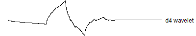
![]()
Now, why the weird appearance? The d4 wavelet optimizes three properties simultaneously. The d4 wavelet chosen to have compact support, both for the wavelet decomposition and the inverse function that reconstructs the wavelet. The d4 wavelet is orthogonal both within a frequency band and across frequency bands. Finally, the d4 wavelet is orthogonal to any linear function, which simplifies the ability of the wavelet transform to isolate linear signals.
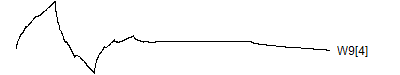
There are four wavelets at this frequency.> graph.single("wave10a.png",wt.comp(wt.rwt,5),"W9[1]")
null device
1
> graph.single("wave10b.png",wt.comp(wt.rwt,6),"W9[2]")
null device
1
> graph.single("wave10c.png",wt.comp(wt.rwt,7),"W9[3]")
null device
1
> graph.single("wave10d.png",wt.comp(wt.rwt,8),"W9[4]")
null device
1
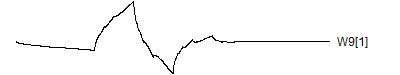
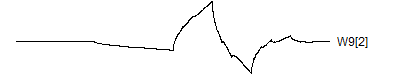
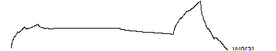
![]()
You'll find out more details about where these wavelet coefficients fit in the wavelet decomposition in little bit. Notice how the last two wavelets wrap around. This is a complication of the edge effects of a signal, and there are several alternative ways to handle these effects: repeat the signal (assuming it is periodic), reflect the signal back, or pad with zeros. The last option is not recommended, and repeating the signal leads to a simple wrap-around effect that is easy to follow.
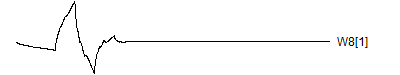
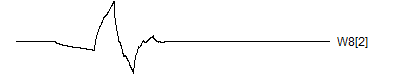
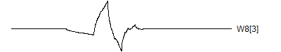
Here are the wavelets at the next higher frequency.
> graph.single("wave11a.png",wt.comp(wt.rwt, 9),"W8[1]")
null device
1
> graph.single("wave11b.png",wt.comp(wt.rwt,10),"W8[2]")
null device
1
> graph.single("wave11c.png",wt.comp(wt.rwt,11),"W8[3]")
null device
1
> graph.single("wave11d.png",wt.comp(wt.rwt,12),"W8[4]")
null device
1
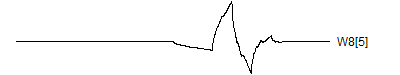
> graph.single("wave11e.png",wt.comp(wt.rwt,13),"W8[5]")
null device
1
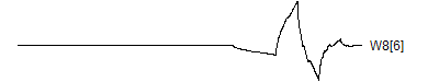
> graph.single("wave11f.png",wt.comp(wt.rwt,14),"W8[6]")
null device
1
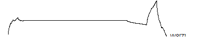
> graph.single("wave11g.png",wt.comp(wt.rwt,15),"W8[7]")
null device
1
> graph.single("wave11h.png",wt.comp(wt.rwt,16),"W8[8]")
null device
1

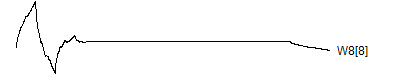
![]()
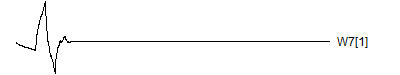
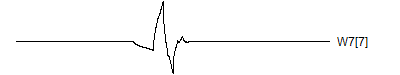
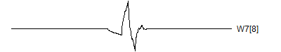
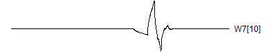
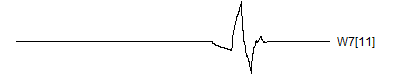
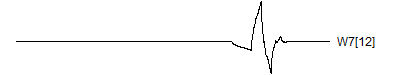
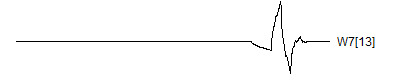
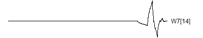
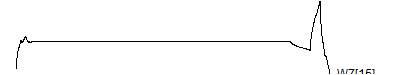
and at the next highest frequency
> graph.single("wave12a.png",wt.comp(wt.rwt,17),"W7[1]")
null device
1
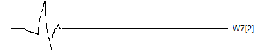
> graph.single("wave12b.png",wt.comp(wt.rwt,18),"W7[2]")
null device
1
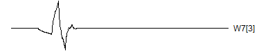
> graph.single("wave12c.png",wt.comp(wt.rwt,19),"W7[3]")
null device
1
> graph.single("wave12d.png",wt.comp(wt.rwt,20),"W7[4]")
null device
1
> graph.single("wave12e.png",wt.comp(wt.rwt,21),"W7[5]")
null device
1
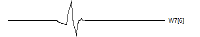
> graph.single("wave12f.png",wt.comp(wt.rwt,22),"W7[6]")
null device
1
> graph.single("wave12g.png",wt.comp(wt.rwt,23),"W7[7]")
null device
1
> graph.single("wave12h.png",wt.comp(wt.rwt,24),"W7[8]")
null device
1
> graph.single("wave12i.png",wt.comp(wt.rwt,25),"W7[9]")
null device
1
> graph.single("wave12j.png",wt.comp(wt.rwt,26),"W7[10]")
null device
1
> graph.single("wave12k.png",wt.comp(wt.rwt,27),"W7[11]")
null device
1
> graph.single("wave12l.png",wt.comp(wt.rwt,28),"W7[12]")
null device
1
> graph.single("wave12m.png",wt.comp(wt.rwt,29),"W7[13]")
null device
1
> graph.single("wave12n.png",wt.comp(wt.rwt,30),"W7[14]")
null device
1
> graph.single("wave12o.png",wt.comp(wt.rwt,31),"W7[15]")
null device
1
> graph.single("wave12p.png",wt.comp(wt.rwt,32),"W7[16]")
null device
1


![]()
Notice that each time the frequency doubles, the number of wavelets also doubles. This creates a pyrimidal cascade of wavelet coefficients.
The calculation of the wavelet decomposition is an interative process. First, you need the coefficients underlying the d4 wavelet. At the highest possible frequency, there are four coefficients.
> g <- d4.rwt$h.0

  > g

    [1]  0.4829629  0.8365163  0.2241439 -0.1294095
These coefficients represent the "high pass" filter. There is a complementary "low pass" filter that you get by reversing the coefficients and changing the sign of every other value.
> h <- d4.rwt$h.1

  > h

[1]  0.1294095  0.2241439 -0.8365163  0.4829629
These two filter pairs are known as a quadrature mirror filter because of the reflection. These two filters are orthonormal.
> dot.prod(g,g)

  [1] 1

  > dot.prod(h,h)

   [1] 1

   > dot.prod(g,h)

    [1] 0
The wavelet decomposition has an overlap, and (thankfully) the first half and the second half pieces are also orthogonal. Remember, orthogonality allows you to derive the mathematical properties of the wavelet decomposition easily and it preserves independence under certain settings.
> dot.prod(g[1:2],g[3:4])

[1] 2.909201e-13

> dot.prod(h[1:2],h[3:4])

[1] 2.909201e-13

> dot.prod(g[1:2],h[3:4])

[1] 0

> dot.prod(h[1:2],g[3:4])

[1] 0
The d4 filter also has one more nice property. The second filter is orthogonal to any linear signal
> dot.prod(h,1:4)

  [1] 1.000117e-12
This means that the linear portion of any signal is not filtered out, but is passed up the ladder of the decomposition. The d6 filter has six coefficients rather than four, and it does not filter out any linear or quadratic signal. The d8 filter has eight coefficients and it does not filter out any linear, quadratic, or cubic signal. In fact, it is this property involving polynomial signals that forms the basis of the Daubechies wavelets.
There's one more property that is not immediately apparent from looking at the d4 wavelet. Some wavelets have simple forms for decomposition, but they get messier for the inverse of the decomposition. The d4 wavelet uses the same number of coefficients (4) in the inverse as it does in the composition. In fact, as you will see below, it uses the exact same vectors.
Let's look at the first level of the wavelet decomposition.
> wt.1 <- mdwt(ecg,g,L=1)

  > V1 <- wt.1$y[   1:1024]

> W1 <- wt.1$y[1025:2048]
For conveniece, split the decomposition into the left half (1:1024) and the right half (1025:2048).
The V1 coefficients represent the running dot product of the signal with the g vector. You skip every other data point in the running dot product, and you rotate the dot product around to the end when reach the right hand side to avoid edge effects. The skipping past the second, fourth, sixth, etc. observation in the running dot product is described in some sources as down-sampling.
> comp(dot.prod(ecg, g,1),V1[1],"V1[1]")

  V1[1]

  By hand -0.1317145

  Using R -0.1317145

 > comp(dot.prod(ecg, g,3),V1[2],"V1[2]")

  V1[2]

  By hand -0.1399428

  Using R -0.1399428

 > comp(dot.prod(ecg, g,5),V1[3],"V1[3]")

  V1[3]

  By hand -0.148171

  Using R -0.148171
The W1 coefficients represent the running dot product of the signal with the h vector, again with downsampling.
> comp(dot.prod(ecg,-h,1),W1[1],"W1[1]")

  W1[1]

  By hand 0.02247964

  Using R 0.02247964

 > comp(dot.prod(ecg,-h,3),W1[2],"W1[2]")

  W1[2]

  By hand 0.02468439

  Using R 0.02468439

 > comp(dot.prod(ecg,-h,5),W1[3],"W1[3]")

  W1[3]

  By hand -0.006023849

  Using R -0.006023849
Notice that you need to negate the h function to get the proper values for W. This is one of those scaling details in wavelets that will drive you nuts.
A second pass applies the same pair of filters to V1. This creates 512 coefficients at the second highest frequency (W2) and 512 coefficients containing everything but W1 and W2 (V2).> wt.2 <- mdwt(ecg,g,L=2)
> V2 <- wt.2$y[ 1: 512]
> W2 <- wt.2$y[513:1024]
Again, for convenience, separate out the first quarter (1:512) and the second quarter (513:1024) of the data.
> comp(dot.prod(V1, g,1),V2[1],"V2[1]")

  V2[1]

  By hand -0.1961169

  Using R -0.1961169

 > comp(dot.prod(V1, g,3),V2[2],"V2[2]")

  V2[2]

  By hand -0.1989215

  Using R -0.1989215

 > comp(dot.prod(V1, g,5),V2[3],"V2[3]")

  V2[3]

  By hand -0.1863624

  Using R -0.1863624
The V2 coefficients represent the running dot product (with downsampling) of V1 and g.
> comp(dot.prod(V1,-h,1),W2[1],"W2[1]")

  W2[1]

  By hand -0.00920762

  Using R -0.00920762

 > comp(dot.prod(V1,-h,3),W2[2],"W2[2]")

  W2[2]

  By hand 0.003389415

  Using R 0.003389415

 > comp(dot.prod(V1,-h,5),W2[3],"W2[3]")

  W2[3]

  By hand -0.0003374554

  Using R -0.0003374554
The W2 coefficients represent the running dot product (with downsampling) of V1 and h.
> all(wt.2$y[1025:2048]==wt.1$y[1025:2048])

  [1] TRUE
The second level of the wavelet decomposition preserves all the W1 coefficients in the back half of the wavelet decomposition.
> wt.2a <- mdwt(V1,g,L=1)

  > length(wt.2a$y)

   [1] 1024

   > all(wt.2a$y==wt.2$y[1:1024])

    [1] TRUE
You get the exact same wavelet decomposition if you apply a level 1 decomposition on V1.
Note the order in which these are stored: 512 V2's at the front, followed by 512 W2's, and 1,024 W1's bring up the rear. You don't need to hang onto V1, because (as we will see in a minute), you can reconstruct the 1.024 V1's from 512 V2's and the 512 W2's. Now, run the wavelet decomposition all the way up to level 3. This creates 256 V3's, 256 W3's, 512 W2's, and 1,024 W1's.
> wt.3 <- mdwt(ecg,g,L=3)

  > W3 <- wt.3$y[257:512]

   > V3 <- wt.3$y[  1:256]
Again for convenience, split apart the decomposition. At this level split into the first eight (1:256) and the second eighth (257:512).
> comp(dot.prod(V2, g,1),V3[1],"V3[1]")

  V3[1]

  By hand -0.28061

  Using R -0.28061

 > comp(dot.prod(V2, g,3),V3[2],"V3[2]")

  V3[2]

  By hand -0.2404948

  Using R -0.2404948

 > comp(dot.prod(V2, g,5),V3[3],"V3[3]")

  V3[3]

  By hand -0.2919882

  Using R -0.2919882
Are you starting to see the pattern? The V3 coefficients represent the running dot product (with downsampling) of V2 and g.
> comp(dot.prod(V2,-h,1),W3[1],"W3[1]")

  W3[1]

  By hand -0.002777659

  Using R -0.002777659

 > comp(dot.prod(V2,-h,3),W3[2],"W3[2]")

  W3[2]

  By hand 0.03857375

  Using R 0.03857375

 > comp(dot.prod(V2,-h,5),W2[3],"W3[3]")

  W3[3]

  By hand  0.0963032950

  Using R -0.0003374554
Ditto for the W3 coefficients.
> all(wt.3$y[ 513:1024]==wt.2$y[ 513:1024])

  [1] TRUE
The W2 coefficients are stored in the same spot for the level 2 and the level 3 decomposition.
> wt.3a <- mdwt(V2,g,L=1)

  > length(wt.3a)

  [1] 2

  > all(wt.3a$y==wt.3$y[1:512])

  [1] TRUE
Finally, you get the exact same values by applying a level 1 decomposition to V2.
You keep on going until you get just about run out of V's.
wt.4 <- mdwt(ecg,g,L=4)

  W4 <- wt.4$y[129:256]

  V4 <- wt.4$y[  1:128]

  wt.5 <- mdwt(ecg,g,L=5)

  W5 <- wt.5$y[ 65:128]

  V5 <- wt.5$y[  1: 64]

  wt.6 <- mdwt(ecg,g,L=6)

  W6 <- wt.6$y[ 33: 64]

  V6 <- wt.6$y[  1: 32]

  wt.7 <- mdwt(ecg,g,L=7)

  W7 <- wt.7$y[ 17: 32]

  V7 <- wt.7$y[  1: 16]

  wt.8 <- mdwt(ecg,g,L=8)

  W8 <- wt.8$y[  9: 16]

  V8 <- wt.8$y[  1:  8]
A level 8 decomposition works pretty well. It has 8 V8's, 8 W8's, 16 W7's, 32 W6's, 64 W5's, 128 W4's, 256 W3's, 512 W2's and 1,024 W1's. The W's store all the information at 8 decreasing frequency levels, and as the frequency decreases from the highest frequency (W1) to lower frequencies, the number of coefficients decreases also. We could take this a couple of steps further, but there is no appreciable benefit to running the wavelet decomoposition all the way to the top, and the edge effects loom very large at the top.
Reconstruction of the original signal works in a similar fashion.
> W8d <- dilute(W8)

  > V8d <- dilute(V8)

   > comp( dot.prod(W8d,g,14)+dot.prod(V8d,h,14),V7[1],"V7[1]")

V7[1]

By hand -3.315508

Using R -3.315508

> comp(-dot.prod(W8d,g,15)-dot.prod(V8d,h,15),V7[2],"V7[2]")

V7[2]

By hand -2.398146

Using R -2.398146

> comp( dot.prod(W8d,g,16)+dot.prod(V8d,h,16),V7[3],"V7[3]")

V7[3]

By hand -0.2769286

Using R -0.2769286

> comp(-dot.prod(W8d,g, 1)-dot.prod(V8d,h, 1),V7[4],"V7[4]")

V7[4]

By hand 1.782748

Using R 1.782748

> comp( dot.prod(W8d,g, 2)+dot.prod(V8d,h, 2),V7[5],"V7[5]")

V7[5]

By hand 5.25007

Using R 5.25007

> comp(-dot.prod(W8d,g, 3)-dot.prod(V8d,h, 3),V7[6],"V7[6]")

V7[6]

By hand 4.7496

Using R 4.7496
You dilute the V8 and W8 coefficients by inserting zeros between every element, compute a running dot product of both the g and the h vectors, and add the results together. For some reason, you have to multiply every other value by -1. I don't know why. It's one of those scaling things. Also notice that you start at almost the very end of V8. This is caused by edge effects.
Once you have V7, repeat the process on the diluted V7 and W7 vectors to get V6.
> W7d <- dilute(W7)

  > V7d <- dilute(V7)

   > comp( dot.prod(W7d,g,30)+dot.prod(V7d,h,30),V6[1],"V6[1]")

V6[1]

By hand -2.096562

Using R -2.096562

> comp(-dot.prod(W7d,g,31)-dot.prod(V7d,h,31),V6[2],"V6[2]")

V6[2]

By hand -2.294492

Using R -2.294492

> comp( dot.prod(W7d,g,32)+dot.prod(V7d,h,32),V6[3],"V6[3]")

V6[3]

By hand -2.441797

Using R -2.441797

> comp(-dot.prod(W7d,g, 1)-dot.prod(V7d,h, 1),V6[4],"V6[4]")

V6[4]

By hand -1.265345

Using R -1.265345

> comp( dot.prod(W7d,g, 2)+dot.prod(V7d,h, 2),V6[5],"V6[5]")

V6[5]

By hand -0.6650157

Using R -0.6650157

> comp(-dot.prod(W7d,g, 3)-dot.prod(V7d,h, 3),V6[6],"V6[6]")

V6[6]

By hand 0.08738041

Using R 0.08738041
And so forth.
> W1d <- dilute(W1)

  > V1d <- dilute(V1)

   > comp( dot.prod(W1d,g,2046)+dot.prod(V1d,h,2046),ecg[1],"ecg[1]")

ecg[1]

By hand -0.104773

Using R -0.104773

> comp(-dot.prod(W1d,g,2047)-dot.prod(V1d,h,2047),ecg[2],"ecg[2]")

ecg[2]

By hand -0.093136

Using R -0.093136

> comp( dot.prod(W1d,g,2048)+dot.prod(V1d,h,2048),ecg[3],"ecg[3]")

ecg[3]

By hand -0.0815

Using R -0.0815

> comp(-dot.prod(W1d,g,   1)-dot.prod(V1d,h,   1),ecg[4],"ecg[4]")

ecg[4]

By hand -0.116409

Using R -0.116409

> comp( dot.prod(W1d,g,   2)+dot.prod(V1d,h,   2),ecg[5],"ecg[5]")

ecg[5]

By hand -0.0815

Using R -0.0815

> comp(-dot.prod(W1d,g,   3)-dot.prod(V1d,h,   3),ecg[6],"ecg[6]")

ecg[6]

By hand -0.116409

Using R -0.116409
At the very end, the calculations on the diluted V1 and W1 values give you the original signal.
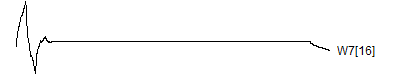
You can see what the wavelet coefficients at each level contribute by zeroing out some of the components and then inverting it.
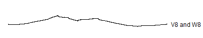
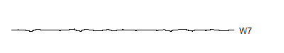
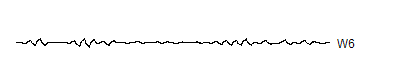
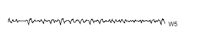
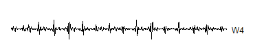
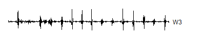
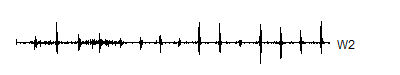
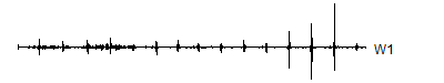
![]()
Notice that the sharp spikes are captured in W1, W2, and W3. The slower overall undulation is captured by V8 and W8. Some of the intermediate squiggles between the sharp spikes are captured in the remaining wavelets.
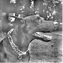
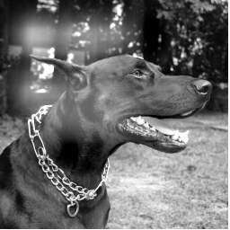
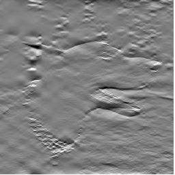
There are simple generalizations of wavelets for two dimensional images. Here's a simple image, which represents a 256 by 256 bit grayscale image of a dog.
img <- read.table("klaus256.txt")

img <- 2*img-1
img.plot <- function(imat,n=256) {

  xsq <- c(0,0,1,1)

  ysq <- c(0,1,1,0)

  par(mar=rep(0,4),xaxs="i",yaxs="i")

  plot(c(1,n+1),c(1,n+1),type="n",axes=FALSE)

  for (i in 1:n) {

  for (j in 1:n){

  d <- 0.5*imat[n+1-j,i]+0.5

  d <- min(1,max(0,d))

  polygon(xsq+i,ysq+j,density=-1,border=NA,col=rgb(d,d,d))

  }

  }

  }
img.plot(img)

Let's also move to a slightly lengthier wavelet, the d8 wavelet.
> g <-  daubcqf(8)$h.0

  > g

   [1]  0.23037781  0.71484657  0.63088077 -0.02798377 -0.18703481  0.03084138

   [7]  0.03288301 -0.01059740

   > h <- -daubcqf(8)$h.1

    > h

     [1] -0.01059740 -0.03288301  0.03084138  0.18703481 -0.02798377 -0.63088077

     [7]  0.71484657 -0.23037781
The d8 wavelet is a bit smoother than d4. It passes linear, quadratic, and cubic functions through to the top of the pyramid, unlike the d4 wavelet which only passes linear functions through. There is slightly greater computational complexity and edge effects can be a bit more pronounced, but these are minor issues.
In one dimention, the d8 wavelet looks like this.
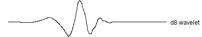
![]()
For a two dimensional image, you take the outer product of g with itself to get an 8 by 8 matrix. This matrix is then slid around on the image to get the V1 coefficients. The W1 coefficents are produced by a similar set of three outer products: the outer product of h with g, the outer product of g with h and the outer product of h with h.
> wt.img.1 <- mdwt(img,g,L=1)

   > comp(sum(img[1:8,1:8]*outer(g,g)),wt.img.1$y[  1,  1],"V1")

V1

By hand -1.580973

Using R -1.580973

> comp(sum(img[1:8,1:8]*outer(h,h)),wt.img.1$y[129,129],"W1")

W1

By hand -0.002825861

Using R -0.002825861

> comp(sum(img[1:8,1:8]*outer(h,g)),wt.img.1$y[129,  1],"W1")

W1

By hand -0.01225749

Using R -0.01225749

> comp(sum(img[1:8,1:8]*outer(g,h)),wt.img.1$y[  1,129],"W1")

W1

By hand -0.005042734

Using R -0.005042734
The first level of the 2D wavelet decomposition for a 256*256 image produces 128*128 V1 coefficients and 3*128*128 W1 coefficients. The second level produces 64*64 V2 coefficients and 3*64*64 W2 coefficients. If you continue this to the sixth level, you get 4*4 V6 coefficients and 3*4*4 W6 coefficients. This continues until the number of V coefficients becomes small. This is a pyrimidal cascade again, but this time a cascade in two dimensions.
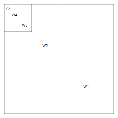
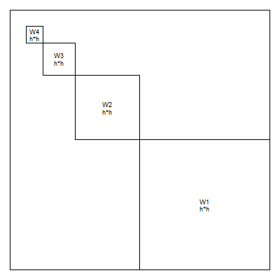
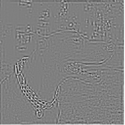
Now there are three different sets of W's, one associated with outer(h,g), one with outer(g,h), and one with outer(h,h). The first represents high frequency changes in the horizontal direction and the second represents high frequency changes in the vertical direction. The third represents high frequency changes in a diagonal direction. In an image, a high frequency event represents a sharp transition between light to dark or dark to light. These transitions frequently represent boundaries or edges in an image.
Although there is some arbitrariness here, you can assign the outer(h,g) wavelets along the top.
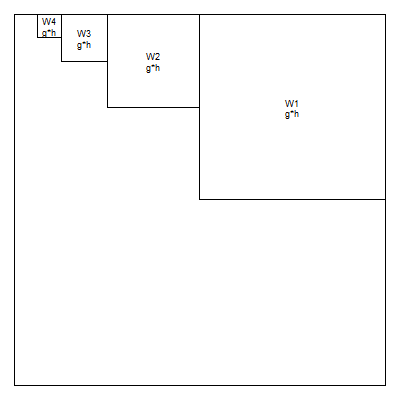
the outer(g,h) wavelets along the side
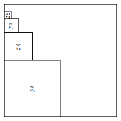
and the outer(h,h) wavelets along the diagonal.
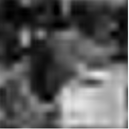
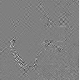
If you examine the contribution of each wavelet frequency to the image, you will see a distinct patter.
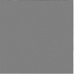
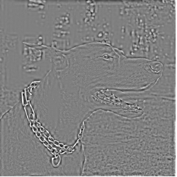
This W1. The gray areas represent the average color and regions of the image where no high frequency events occur. You can see high frequency events around the dog's collar and the dog's face.
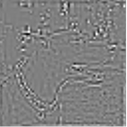
This is W2. It looks a lot like W1 but is a bit broader.
This is W3. You see a bit more activity in the background, representings shifts in the color of the background image.
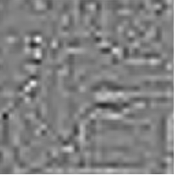
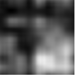
This is W4. It looks like a blurred image with undulating colors rather than sharp shifts.
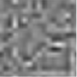
This is W5. It is an amorphous blob representing graduals shifts in the average color.
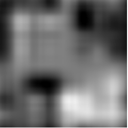
This is W6. It is just like W5 at an even broader scale.
If you look at the original image again, you will see regions (mostly in the background surrounding the dog or in large patches of the dog's fur) where the color is mostly the same. These are captured by the low frequency wavelets. The sudden transitions in color, especially around the dog's collar, are captured in high frequency wavelets. You can look at the cumulative effect of the wavelets as well.
Here is W1 again.
Here is W1 plus W2.
Here is W1 through W3. Notice that the edges around the collar and the dog's face are well defined here. Also notice the large patches of gray. Gray is zero and it represents the average color between white and black. The areas in gray have no sharp edges and are filled in primarily with the lower frequency wavelets.
Here is W1 through W4. At this level, some of the broad color regions are starting to become apparent, though the image is still largely washed out.
Here is W1 through W5. The image is very similar to the original, but there are some patches that V5 would be needed to fill in.
You can also look at the reconstructed image using V1 through V6.

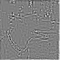
Here is V1. It is the full image with just a few very sharp edges removed by W1.
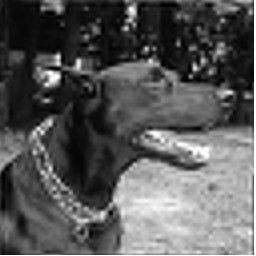
Here is V2. With removal of another set of edges by W2, the picture starts to take on a slightly blurry feel.

Here is V3. It has an even greater blur.
Here is V4. The dog is blurred almost beyond recognition.
Here is V5. There is nothing recognizable here except general patterns of dark and light through broad regions of the image.

Finally, here is V6. It is pretty much the same as V6, but at an even broader scale.
You can also reconstruct the three different sets of wavelet coefficients separately.
Here is an image reconstructed with the W1 through W3 of horizontally oriented wavelets only.

Here is the reconstruction using W1 through W3 of the vertically oriented wavelets only.
Here is the reconstruction using W1 through W3 of the diagonally oriented wavelets only.
There seems to be more detail in the horizontally oriented wavelets. That's because the mouth, the eye and the ear are mostly horizontal. The edge of the dog's body, however, is vertical and is prominent only in the second image. The collar is a mix of horizontal, vertical, and diagonal elements, so it is apparent in each of the three images.
There's a lot more to wavelets, but this should help get you started. Now that you know how to compute the wavelet decomposition in one and two dimensions, you are ready to start applying them to real situations.
There are several important applications of wavelets. First, the wavelet coefficients themselves tell you information about the nature of the signal or image. Are there high frequency events or low frequency events (or both) and are those restricted to a particular part of the signal.
Second, you can use wavelets to get a "de-noised" signal. Those small coefficients that are (presumably) just noise. If you reconstruct the signal or image without those small coefficients (by rounding them down to zero), you will often get a "cleaner" estimate of the signal. Wavelets do an especially good job of de-noising when the signal is not smooth. Smooth means a discontinuous first derivative, but in most applications it represents an abrupt turn in the signal. Wavelets even can work well with discontinuous signals.
In contrast, the Fourier decomposition has lots of problems with non-smooth, but especially discontinuous functions. The problems go under the general name of the Gibbs phenomenon.
Third, you can zero out the small coefficients and store only the large coefficients. This allows you to reconstruct a good approximation of the image while saving substantially on storage. This is really only used for images, because one dimensional signals, even very long ones just don't take up a lot of room. The jpg 2000 standard used wavelets for compression.
Fourth, wavelets can help you detect edges in an image. An edge is an abrupt transition from light to dark, or dark to light. The high frequency wavelets help you detect where the edges are in an image.
Wavelets have a couple important limitations. The first is a minor issue, but the wavelets need to be adapted when the number of points in your signal is not a simple power of 2 or when the two dimensions of length and width of your image are not both simple powers of 2. A more important problem is that wavelets rely on equally spaced sample of the signal or image. Subsampling or interpolation can sometimes help here.
![]() This page was written by
Steve Simon and is licensed under the Creative
Commons Attribution 3.0 United States License. Need more
information? I have a page with general help
resources.
This page was written by
Steve Simon and is licensed under the Creative
Commons Attribution 3.0 United States License. Need more
information? I have a page with general help
resources.