![]()
StATS: What is a decision rule?Hypotheses, errors, and decision rules.
In this section, we discuss the basic components needed for testing: hypotheses, error types, and decision rules. There are two types of hypotheses, the null and alternate hypothesis. The null hypothesis is the “status quo” hypothesis: the hypothesis that includes equality.
There are two types of errors. Type I errors are comparable to allowing an ineffective drug onto the market. Type II erros are comparable to keeping an effective drug off the market.
The decision rule compares the sample mean to the hypothesized mean. If the sample mean is "close" to the hypothesized mean, we accept the null hypothesis.
Hypotheses
Before we can perform a statistical test, we need a pair of hypothesis. By tradition, we call the hypothesis that includes equality as the null hypothesis.
A research hypothesis is a statement about a population parameter. Here are some examples. The average waiting time for all patients in the Emergency Room is equal to 55 minutes
The average weight of all babies of 32 weeks gestational age is less than 1800 grams.
The null and alternative hypotheses.
We will label the research hypothesis using H0 and a counterpart to this hypothesis as H1. H0 is called the null hypothesis; H1 the alternative hypothesis. Traditionally, H0 is the hypothesis that includes equality.
When our alternative hypotheses uses a "not equal to" sign, we refer to the hypothesis as a two directional or a two tailed hypothesis.
An arbitrary decision rule.
We will use information from a sample to decide among the two hypotheses. In general, if XBAR is close to the hypothesized mean, we would accept H0. If XBAR is far away from the hypothesized mean, then we would reject H0.
For example, for the hypotheses
we might try the following rule:
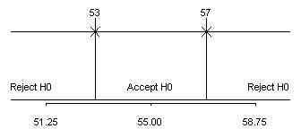
Accept H0 if XBAR is between 53 and 57, otherwise reject H0.
Note that this is a very arbitrary rule.
Definition of Type I and Type II errors.
Sometimes our decisions will be correct and sometimes not. There are two possible errors, which we will call Type I and Type II errors, respectively.
A Type I error, a false positive conclusion, is rejecting H0 when H0 is true. A Type II error, a false negative conclusion, is accepting H0 when H0 is false.
In many hypothesis testing situations, a hypothesis test will be used to decide whether to change to a new drug or therapy. Decision: change if we reject H0; don’t change if we accept H0. In such a situation, a Type I error is allowing an ineffective product onto the market. A Type II error is keeping an effective product off the market.
Definition of Alpha and Beta.
While we can’t prevent the possibility of incorrect decisions, we can try to minimize their probabilities. We will refer to alpha and beta as the probabilities of Type I and Type II errors, respectively.
Alpha=P[Type I error] = P[Reject H0 | H0 true]
Beta=P[Type II error] = P[Accept H0 | H0 false]
Calculating Alpha.
Normally, we don’t calculate alpha. But it is a way of assessing the quality of an arbitrary decision rule. Suppose we have the following hypothesis
[insert hypothesis]
and decision rule
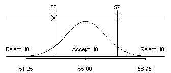
Accept H0 if XBAR is between 53 and 57, otherwise reject H0.
If the sample size is 504 and sigma = 28, then compute alpha.
With the arbitrary decision rule given above, there is about an 11% chance of rejecting H0 when H0 is true.
Decision rules.
A decision rule uses information from a sample to make a choice between two hypotheses. In this section, we will learn how to create decision rules that keep the probability of a Type I error reasonably small.
Creating a decision rule for a two tailed test.
Suppose we want to test the two tailed hypothesis
We also want to hold the probability of a Type I error to a small value (alpha). Then our decision rule ought to be reject H0 if
or if
Example of a decision rule for a two tailed test.
Create a decision rule for:
Suppose we want alpha=.05. Also suppose that
Our decision rule is reject H0 if
or if
Since XBAR is between 52.55 and 57.45, we accept H0. We conclude that the average waiting time for all patients in the Emergency Room is 55 minutes. We will show equivalent ways to test this hypothesis in sections 2.1.5 and 2.2.4.
A second example.
Create a decision rule for:
Suppose we want alpha=.10. Also suppose that
Note here that the assumption of normality is important. Our decision rule is reject H0 if
or if
Since XBAR is less than 1699.2, we reject H0. We conclude that the average weight of all 32 week gestational age babies is not equal to 1800 grams. We will show equivalent ways to test this hypothesis in sections 2.1.3 and 2.2.3.
Relationship to confidence intervals.
Suppose we are testing a two sided hypothesis. Our decision rule would be to reject H0 if
or if
Equivalently, we could use the following decision rule: reject H0 if
or if
The limits above are the limits of a 1-alpha confidence interval. So we can re-write this decision rule as
Reject H0 if the 1-alpha confidence interval does not contain mu0.
Examples of using confidence intervals to test hypotheses.
The 95% confidence for the data given in section 1.3.2 is
(53.66,58.54).
Since this interval contains 55, we accept H0.
The 90% confidence interval for the data given in section 1.3.3 is
(1596.2,1797.8)
Since this interval does not contain 1800, we reject H0.
Summary.
What have we learned so far?
The three types of hypotheses. left, right, and two tailed. The two types of errors. How to construct a decision rule that minimizes the probability of a Type I error. 1.9.1 Group exercise
Practice exercise
The following data are readability levels for a random sample of 30 informational pamphlets on cancer.
8, 7, 6, 11, 10, 8, 14, 15, 9, 12, 13, 6, 9, 8, 8, 6, 9, 8, 12, 12, 12, 15, 8, 7, 7, 16, 8, 13, 8, 9
Enter these data into SPSS and compute the mean and standard deviation. Test the hypothesis that the average readability level of all informational pamphlets is at the 8th grade level. Use an alpha level of .01.
The following data are readability levels for 63 patients with cancer. Enter these data into SPSS and compute the mean and standard deviation. Test the hypothesis that the average readability level of all cancer patients is at the 8th grade level. Use an alpha level of .01.
11, 8, 4, 9, 10, 11, 9, 13, 11, 7, 13, 2, 13, 6, 9, 13, 13, 2, 8, 4, 11, 10, 13, 13, 13, 12, 2, 3, 2, 13, 6, 9, 8, 8, 3, 13, 13, 13, 2, 12, 10, 10, 8, 13, 3, 7, 5, 13, 11, 4, 13, 8, 13, 11, 6, 5, 9, 3, 5, 11, 13, 4, 2
Source: http://www.stat.ncsu.edu/info/jse/datasets.index.html Journal of Statistics Education Data Archive.
This page was written by Steve Simon while working at Children's Mercy Hospital. Although I do not hold the copyright for this material, I am reproducing it here as a service, as it is no longer available on the Children's Mercy Hospital website. Need more information? I have a page with general help resources. You can also browse for pages similar to this one at Category: Definitions, Category: Hypothesis testing.