
The concepts behind the logistic regression model (July 23, 2002)
This page is moving to a new website.
The logistic regression model is a model that uses a binary (two possible values) outcome variable. Examples of a binary variable are mortality (live/dead), and morbidity (healthy/diseased). Sometimes you might take a continuous outcome and convert it into a binary outcome. For example, you might be interested in the length of stay in the hospital for mothers during an unremarkable delivery. A binary outcome might compare mothers who were discharged within 48 hours versus mothers discharged more than 48 hours.
The covariates in a logistic regression model represent variables that might be associated with the outcome variable. Covariates can be either continuous or categorical variables.
For binary outcomes, you might find it helpful to code the variable using indicator variables. An indicator variable equals either zero or one. Use the value of one to represent the presence of a condition and zero to represent absence of that condition. As an example, let 1=diseased, 0=healthy.
Indicator variables have many nice mathematical properties. One simple property is that the average of an indicator variable equals the observed probability in your data of the specific condition for that variable.
A logistic regression model examines the relationship between one or more independent variable and the log odds of your binary outcome variable. Log odds seem like a complex way to describe your data, but when you are dealing with probabilities, this approach leads to the simplest description of your data that is consistent with the rules of probability.
Let's consider an artificial data example where we collect data on the gestational age of infants (GA), which is a continuous variable, and the probability that these infants will be breast feeding at discharge from the hospital (BF), which is a binary variable. We expect an increasing trend in the probability of BF as GA increases. Premature infants are usually sicker and they have to stay in the hospital longer. Both of these present obstacles to BF.
A linear model for probability
A linear model would presume that the probability of BF increases as a linear function of GA. You can represent a linear function algebraically as
prob BF = a + b*GA
This means that each unit increase in GA would add b percentage points to the probability of BF. The table shown below gives an example of a linear function.
This table represents the linear function
prob BF = 4 + 2*GA
which means that you can get the probability of BF by doubling GA and adding 4. So an infant with a gestational age of 30 would have a probability of 4+2*30 = 64.
A simple interpretation of this model is that each additional week of GA adds an extra 2% to the probability of BF. We could call this an additive probability model.
I'm not an expert on BF; what little experience I've had with the topic occurred over 40 years ago. But I do know that an additive probability model tends to have problems when you get probabilities close to 0% or 100%. Let's change the linear model slightly to the following:
prob BF = 4 + 3*GA
This model would produce the following table of probabilities.
You may find it difficult to explain what a probability of 106% means. This is a reason to avoid using a additive model for estimating probabilities. In particular, try to avoid using an additive model unless you have good reason to expect that all of your estimated probabilities will be between 20% and 80%.
A multiplicative model for probability
It's worthwhile to consider a different model here, a multiplicative model for probability, even though it suffers from the same problems as the additive model.
In a multiplicative model, you change the probabilities by multiplying rather than adding. Here's a simple example.
In this example, each extra week of GA produces a tripling in the probability of BF. Contrast this to the linear models shown above, where each extra week of GA adds 2% or 3% to the probability of BF.
A multiplicative model can't produce any probabilities less than 0%, but it's pretty easy to get a probability bigger than 100%. A multiplicative model for probability is actually quite attractive, as long as you have good reason to expect that all of the probabilities are small, say less than 20%.
The relationship between odds and probability
Another approach is to try to model the odds rather than the probability of BF. You see odds mentioned quite frequently in gambling contexts. If the odds are three to one in favor of your favorite football team, that means you would expect a win to occur about three times as often as a loss. If the odds are four to one against your team, you would expect a loss to occur about four times as often as a win.
You need to be careful with odds. Sometimes the odds represent the odds in favor of winning and sometimes they represent the odds against winning. Usually it is pretty clear from the context. When you are told that your odds of winning the lottery are a million to one, you know that this means that you would expect to having a losing ticket about a million times more often than you would expect to hit the jackpot.
It's easy to convert odds into probabilities and vice versa. With odds of three to one in favor, you would expect to see roughly three wins and only one loss out of every four attempts. In other words, your probability for winning is 0.75.
If you expect the probability of winning to be 20%, you would expect to see roughly one win and four losses out of every five attempts. In other words, your odds are 4 to 1 against.
The formulas for conversion are
odds = prob / (1-prob)
and
prob = odds / (1+odds).
In medicine and epidemiology, when an event is less likely to happen and more likely not to happen, we represent the odds as a value less than one. So odds of four to one against an event would be represented by the fraction 1/4 or 0.25. When an event is more likely to happen than not, we represent the odds as a value greater than one. So odds of three to one in favor of an event would be represented simply as an odds of 3. With this convention, odds are bounded below by zero, but have no upper bound.
A log odds model for probability
Let's consider a multiplicative model for the odds (not the probability) of BF.
This model implies that each additional week of GA triples the odds of BF. A multiplicative model for odds is nice because it can't produce any meaningless estimates.
It's interesting to look at how the logarithm of the odds behave.
Notice that an extra week of GA adds 1.1 units to the log odds. So you can describe this model as linear (additive) in the log odds. When you run a logistic regression model in SPSS or other statistical software, it uses a model just like this, a model that is linear on the log odds scale. This may not seem too important now, but when you look at the output, you need to remember that SPSS presents all of the results in terms of log odds. If you want to see results in terms of probabilities instead of logs, you have to transform your results.
Let's look at how the probabilities behave in this model.
Notice that even when the odds get as large as 27 to 1, the probability still stays below 100%. Also notice that the probabilities change in neither an additive nor a multiplicative fashion.
A graph shows what is happening.
The probabilities follow an S-shaped curve that is characteristic of all logistic regression models. The curve levels off at zero on one side and at one on the other side. This curve ensures that the estimated probabilities are always between 0% and 100%.
An example of a log odds model with real data
There are other approaches that also work well for this type of data, such as a probit model, that I won't discuss here. But I did want to show you what the data relating GA and BF really looks like.
I've simplified this data set by removing some of the extreme gestational ages. The estimated logistic regression model is
log odds = -16.72 + 0.577*GA
The table below shows the predicted log odds, and the calculations needed to transform this estimate back into predicted probabilities.
Let's examine these calculations for GA = 30. The predicted log odds would be
log odds = -16.72 + 0.577*30 = 0.59
Convert from log odds to odds by exponentiating.
odds = exp(0.59) = 1.80
And finally, convert from odds back into probability.
prob = 1.80 / (1+1.80) = 0.643
The predicted probability of 64.3% is reasonably close to the true probability (77.8%).
You might also want to take note of the predicted odds. Notice that the ratio of any odds to the odds in the next row is 1.78. For example,
3.20/1.80 = 1.78
5.70/3.20 = 1.78
It's not a coincidence that you get the same value when you exponentiate the slope term in the log odds equation.
exp(0.59) = 1.78
This is a general property of the logistic model. The slope term in a logistic regression model represents the log of the odds ratio representing the increase (decrease) in risk as the independent variable increases by one unit.
Categorical variables in a logistic regression model
You treat categorical variables in much the same way as you would in a linear regression model. Let's start with some data that listed survival outcomes on the Titanic. That ship was struck by an iceberg and 863 passengers died out of a total of 1,313. This happened during an era where there was a strong belief in "women and children" first.
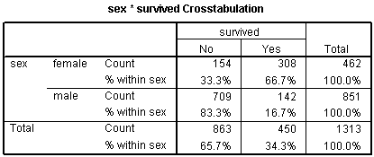
You can see this in the crosstabulation shown above. Among females, the odds of dying were 2-1 against, because the number of survivors (308) was twice as big as the number who died (154). Among males, the odds of dying were almost 5 to 1 in favor (actually 4.993 to 1), since the number who survived (142) was about one-fifth the number who died (709).
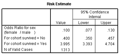
The odds ratio is 0.1, and we are very confident that this odds ratio is less than one, because the confidence interval goes up to only 0.13. Let's analyze this data by creating an indicator variable for sex.
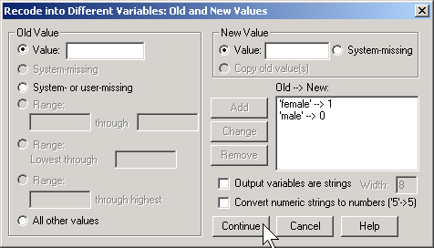
In SPSS, you would do this by selecting TRANSFORM | RECODE from the menu
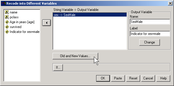
Then click on the OLD AND NEW VALUES button.
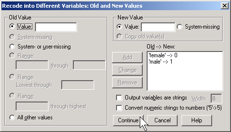
Here, I use the codes of 0 for female and 1 for male. To run a logistic regression in SPSS, select ANALYZE | REGRESSION | BINARY LOGISTIC from the menu.
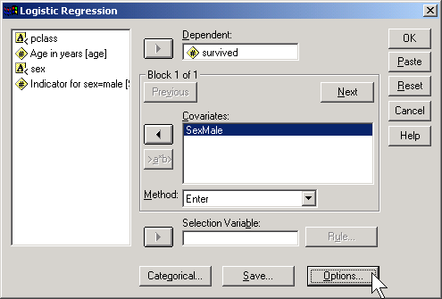
Click on the OPTIONS button.
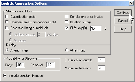
Select the CI for exp(B) option, then click on the CONTINUE button and then on the OK button. Here is what the output looks like:

Let's start with the CONSTANT row of the data. This has an interpretation similar to the intercept in the linear regression model. the B column represents the estimated log odds when SexMale=0. Above, you saw that the odds for dying were 2 to 1 against for females, and the natural logarithm of 2 is 0.693. The last column, EXP(B) represents the odds, or 2.000. You need to be careful with this interpretation, because sometimes SPSS will report the odds in favor of an event and sometimes it will report the odds against an event. You have to look at the crosstabulation to be sure which it is.
The SexMale row has an interpretation similar to the slope term in a linear regression model. The B column represents the estimated change in the log odds when SexMale increases by one unit. This is effectively the log odds ratio. We computed the odds ratio above, and -2.301 is the natural logarithm of 0.1. The last column, EXP(B) provides you with the odds ratio (0.100).
Coding is very important here. Suppose you had chosen the coding for SexFemale where1=female and 0=male.
Then the output would look quite different.

The log odds is now -1.608 which represents the log odds for males. The log odds ratio is now 2.301 and the odds ratio is 9.986 (which you might want to round to 10).
SPSS will create an indicator variable for you if you click on the CATEGORICAL button in the logistic regression dialog box.
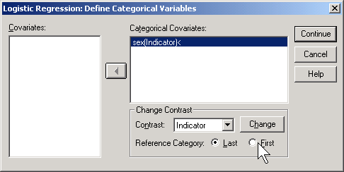
If you select LAST as the reference category, SPSS will use the code 0=male, 1=female (last means last alphabetically). If you select FIRST as the reference category, SPSS will use the code 0=female, 1=male.
How would SPSS handle a variable like Passenger Class, which has three levels
- 1st,
- 2nd,
- 3rd?
Here's a crosstabulation of survival versus passenger class.
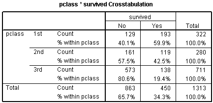
Notice that the odds of dying are 0.67 to 1 in 1st class, 1.35 to 1 in 2nd class, and 4.15 to 1 in 3rd class. These are odds in favor of dying. The odds against dying are 1.50 to 1, 0.74 to 1, and 0.24 to 1, respectively.

The odds ratio for the pclass(1) row is 6.212, which is equal to 1.50 / 0.24. You should interpret this as the odds against dying are 6 times better in first class compared to third class. The odds ratio for the pclass(2) row is 3.069, which equals 0.74 / 0.24. This tells you that the odds against dying are about 3 times better in second class compared to third class. The Constant row tells you that the odds are 0.241 to 1 in third class.
If you prefer to do the analysis with each of the other classes being compared back to first class, then select FIRST for reference category.
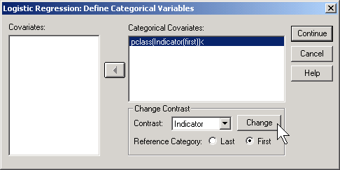
This produces the following output:

Here the pclass(1) row provides an odds ratio of 0.494 which equals 0.74 / 1.50. The odds against dying are about half in second class versus first class. The pclass(2) provides an odds ratio of 0.161 (approximately 1/6) which equals 0.24 / 1.50. The odds against dying are 1/6 in third class compared to first class. The Constant row provides an odds of 1.496 to 1 against dying for first class.
Notice that the numbers in parentheses (pclass(1) and pclass(2)) do not necessarily correspond to first and second classes. It depends on how SPSS chooses the indicator variables. How did I know how to interpret the indicator variables and the odds ratios? I wouldn't have known how to do this if I hadn't computed a crosstabulation earlier. It is very important to do a few simple crosstabulations before you run a logistic regression model, because it helps you orient yourself to the data.
Looking at a variable both continuously and categorically.
Suppose you wanted to further explore the concept of "women and children first" by looking at how age affects the odds against survival. Here is a simple model that includes age as a continuous variable:

The odds ratio for age is 0.991. This tells you that the odds against dying drop by about 1% for each year of life. In other words, the older you are the more likely you are to die. Let's re-interpret this in terms of decades. A full decade change in age would lead to a -0.009 * 10 unit change in the log odds ratio. This leads to an odds ratio of 0.91 per decade, which says the odds against dying decline by about 9% for each extra decade of life.
I have a problem with this model, because it assumes that the effect of one year of age is the same for children, teenagers, adults, and very old people. I suspect that perhaps the effect of age is very strong for young people but it levels off in adults. The chances of dying for a 30 year old would probably not be too much different than for a 40 year old. Let's split the data into different age groups and see how each of them compares.
To do this in SPSS, select TRANSFORM | RANK CASES from the menu.

Click on the RANK TYPES button.

Select Ntiles and choose 10 for the number of groups. This is a somewhat arbitrary choice. You want enough groups to allow for subtle changes across the age range, but if there are too many groups, you lose too much precision.

Here's what you get

Notice that the first group has an average age of 6.6. We'll call those the young children. The next group has an average age of 17.9 which looks more like older teenagers. The remaining groups represent adults of various ages. We have about 70-80 people in each age group. Here is a crosstabulation of age groups by survival.

Notice that the chances for survival are best for the young children. Survival also seems to be high for older teenagers and some of the older adult categories. The worst survival rates are in age groups 3, 4, 5, 6, and 8. Perhaps there is some tendency in this data for "women, children, and old people" first. Here's what a logistic regression model looks like for age groups.

All age groups have a decreased chance of surviving relative to the young children group. You might want to investigate this further looking at combining some or all of the adult groups and splitting the young children group into further subcategories.